Information theory 3: channel coding

7.9k words, including equations (~41 minutes)

 

We've looked at basic information theory concepts here, and at source coding (i.e. compressing data without caring about noise) here. Now we turn to channel coding.

The purpose of channel coding is to make information robust against any possible noise in the channel.

Noisy channel model

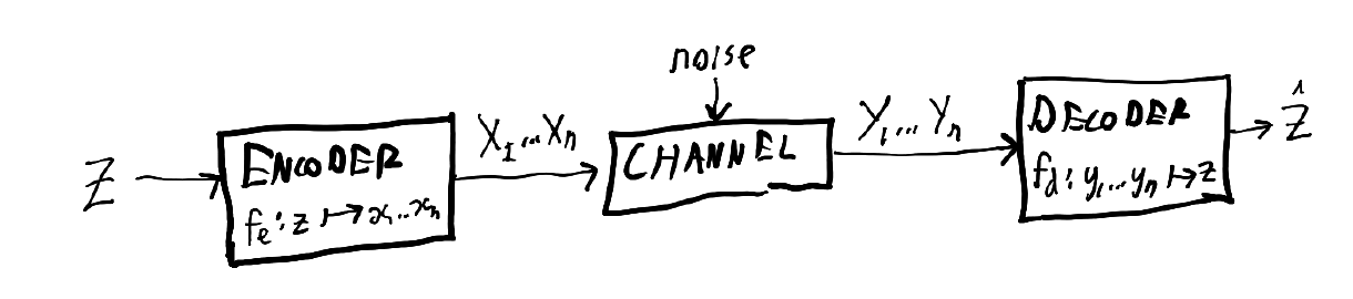
The noisy channel model looks like the following:

The channel can be anything: electronic signals sent down a wire, messages sent by post, or the passage of time. What's important is that it is discrete (we will look at the continuous case later), and there are some transition probabilities from every symbol that can go into the channel to every symbol that can come out. Often, the set of symbols of the inputs is the same as the set of symbols of the outputs.

The capacity $$C$$ of a noisy channel is defined as $$$ C = \max_{p_x} I(X;Y) = \max_{p_x} \big(H(Y) - H(Y|X)\big). $$$ It's intuitive that this definition involves the mutual information $$I$$ (see the first post for the definition and explanation), since we care about how much information $$X$$ transfers to $$Y$$, and how much $$Y$$ tells us about $$X$$. What might be less obvious is why we take the maximum over possible input probability distributions $$p_x$$. This is because the mutual information $$I(X;Y)$$ depends on the probability distributions of $$X$$ and $$Y$$. We can only control what we send - $$X$$ - so we want to adjust that to maximise the mutual information. Intuitively, if you're typing on a keyboard with all keys working normally except the "i" key results in a random character being inserted, shifting your typing away from using the "i" key is good for information transfer. Better to wr1te l1ke th1s than to not be able to reliably transfer information.

However, the only real way to understand why this definition makes sense is to look at the noisy channel coding theorem. This theorem tells us, among other things, that for any rate (measured in bits per symbol) smaller than the capacity $$C$$, for a large enough code length we can get a probability of error as small as we like.

With noisy channels, we often work with block codes. The idea is that you encode some shorter sequence of bits as a longer sequence of bits, and if you've designed this well, it adds redundancy. An $$(n,k)$$ block code is one that replaces chunks of $$k$$ bits with chunks of $$n$$ bits.

Hamming coding

Before we look at the noisy channel theorem, here's a simple code that is redundant to error: transmit every bit 3 times. Instead of sending 010, send 000111000. If the receiver receives 010111000, they can tell that bit 2 probably had an error, and should be a zero. The problem is that you triple your message length.

Hamming codes are a method for achieving the same - the ability to detect and correct single-bit errors, and the ability to detect but not properly correct two-bit errors - while sending a number of excess bits that grows only logarithmically with message length. For long enough messages, this is very efficient; if you're sending over 250 bits, it only costs you a 3% longer message to insure them against single-bit errors.

The catch is that the probability of having only one or fewer errors in a message declines exponentially with message length, so this is less impressive than it might sound at first.

The basic idea of most error correction codes is a parity bit. A parity bit $$b$$ is typically the XOR (exclusive-or) of a bunch of other bits $$b_1, b_2, \ldots$$, written $$b = b_1 + b_2 + \ldots$$ (we use $$+$$ for XOR because doing addition in base-2 while throwing away the carry is the same is taking the XOR). A parity bit over a set of bits $$B = {b_1, b_2, \ldots}$$ is 1 if the set of bits contains an odd number of 1s, and otherwise 0 (hence the word "parity").

Consider sending a 3-bit message where the first two bits are data and the third is a parity bit. If the message is 110, we check that, indeed, there's an even number of 1s among the data bits, so it checks out that the parity bit is 0. If the message were 111, we'd know that something had gone wrong (though we wouldn't be able to fix it, since it could have started out with any of 011, 101, or 110 and suffered a one-bit flip - and note that we can never entirely rule out that 000 flipped to 111, though since error probability is generally small in any case we're interested in, this would be extremely unlikely).

The efficiency of Hamming codes comes from the fact that we have parity bits that check other parity bits.

A $$(T, D)$$ Hamming code is one that sends $$T$$ bits in total of which $$D$$ are data bits and the remaining $$T - D$$ are parity bits. There exists a $$(2^m - 1, 2^m - m - 1)$$ Hamming code for positive integer $$m$$. Note that $$m$$ is the number of parity bits.

The default way to construct a Hamming code is that the $$m$$th parity bit is in position $$2^m - 1$$, and is set such that the parity of bits whose position's binary representation has a 1 in the $$m$$th last position is zero.

(Above, you see bits 1 through 15, with parity bits in positions 1, 2, 4, and 8. Underneath each bit, for every parity bit there is a 0 if that bit is not included in the parity set of that parity bit, and otherwise a 1. For example, since b4 is set for bits 8-15, b4 is a 1 if there's an odd number of 1s in bits 8-15 inclusive and otherwise 0. Note that the columns spell out the numbers 1 through 15 in binary.)

For example, a $$(7,4)$$ Hamming code for the 4 bits of data 0101 would first become $$$ \texttt{ b1 b2 0 b3 1 0 1} $$$ and then we'd set $$b_1 = 0$$ to make there be an even number of 1s across the 1st, 3rd, 5th, and 7th positions, set $$b_2 = 1$$ to do the same over the 2nd, 3rd, 6th, and 7th positions, and then finally set $$b_3 = 0$$ to do the same over the 4th, 5th, 6th, and 7th positions.

To correct errors, we have the following rule: sum up the positions of the parity bits that do not match. For example, if parity bit 3 is set wrong relative to the rest of the message, you flip that bit; everything will be fine after we clear this false alarm. But if parity bit 2 is also set wrong, then you take their positions, 2 (for bit 2) and 4 (for bit 3) and add them to get 6, and flip the sixth bit to correct the error. This makes sense because the sixth bit is the only bit covered by both parity bits 2 and 3, and only parity bits 2 and 3.

Though the above scheme is elegant and extensible, it's possible to design other Hamming codes. The length requirements remain - the code is a $$(2^m - 1, 2^m - m - 1)$$ code if we allow $$m$$ parity bits - but we can assign any "domain" over the bits to each parity bit as long as each bit belongs to the domain a unique set of parity bits.

Noisy channel coding theorem

We can measure any noisy channel code we choose based on two numbers. The first is its probability of error ($$p_e$$ above). The second is its rate: how many bits of information are transferred for each symbol sent. The three parts of the theorem combine to divide that space up into a possible and impossible region:

The first part of the theorem says that the region marked "I" is possible. Now there are points of this region that are more interesting than others. Yes, we can make a code that has a capacity of 0 and a very high error rate; just send the same symbol all the time. This is point (a), and we don't care about it.

What's more interesting, and perhaps not even intuitively obvious at all, is that we can get to a point (b): an arbitrarily low error rate, despite the fact that we're sending information. The maximum information rate we can achieve while keeping the error probability very low turns out to be the capacity, $$C = \max_{p_X} I(X:Y)$$.

The second part of the theorem gives us a lower bound on error rate if we dare try for a rate that is greater than the capacity. It tells us we can make codes that achieve point (c) on the graph.

Finally, the third part of the theorem proves that we can't get to points like (x), that have an error rate that is too low given how much over the channel capacity their rate is.

We started the proof of the source coding theorem by considering a simple construction (the $$\delta$$-sufficient subset) first for a single character and then extending it to blocks. We're going to do something similar now.

Noisy typewriters

A noisy typewriter over the alphabet $${0, \ldots, n}$$ is a device where if you press the key for $$i$$, it inputs one of the following with equal probability:

• $$i - 1 \mod n$$
• $$i \mod n$$
• $$i + 1 \mod n$$

With a 6-symbol alphabet, we can illustrate its transition probability matrix as a heatmap:

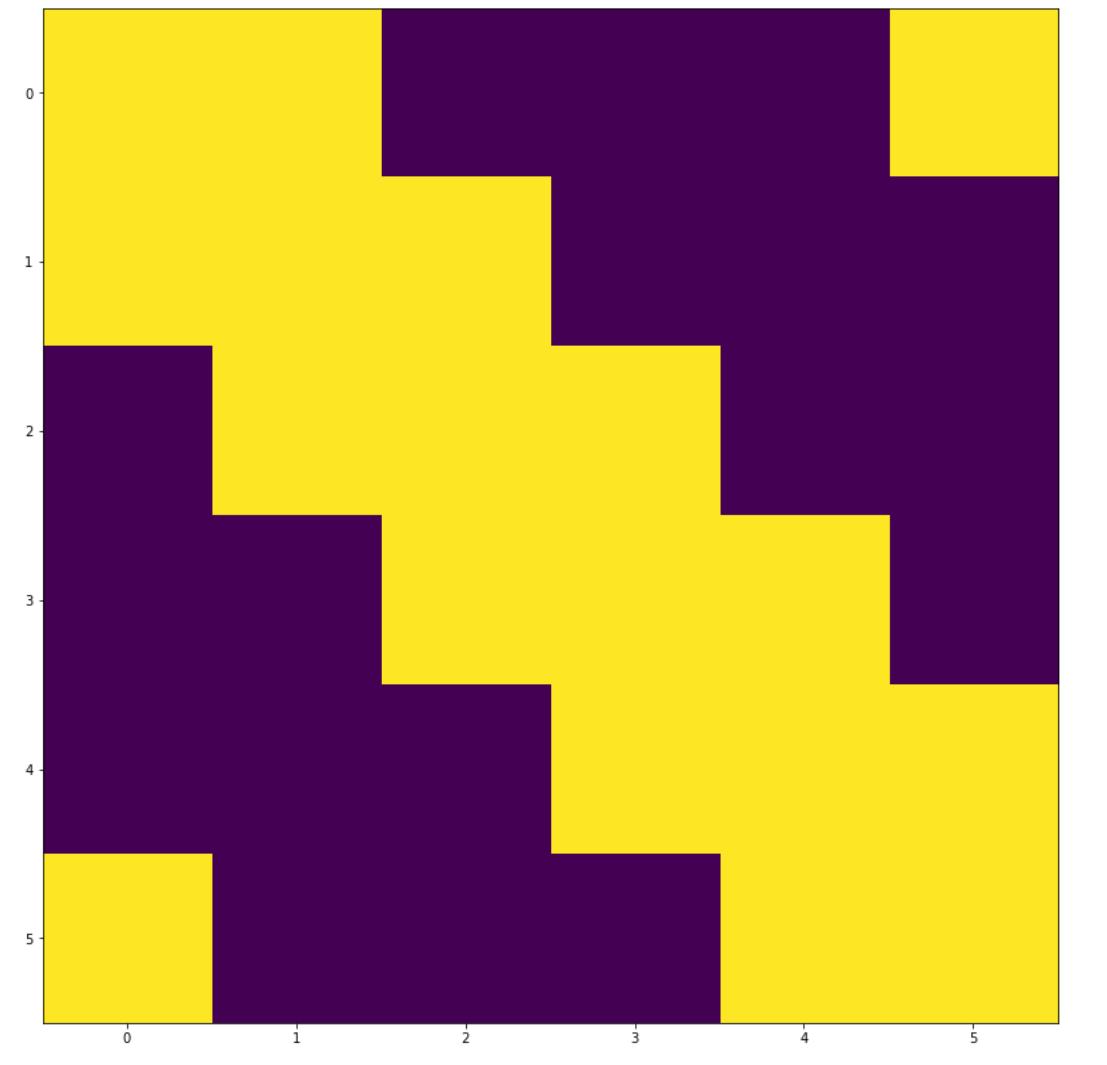
The colour scale is blue (low) to yellow (high). The reading order is meant to be that each column represents the probability distribution of output symbols given an input symbol.

First, can we transmit information without error at all? Yes: choose a code where you only send the symbol corresponding to the second and fifth columns. Based on the heatmap, these can map to symbols number 1-3 and 4-6 respectively; there is no possibility of confusion. The cost is that instead of being able to send one of six symbols, or $$\log 6$$ bits of information per symbol, we can now only send one of two, or $$\log 2 = 1$$ bits of information per symbol.

The capacity is $$\max_{p_X} \big( H(Y) - H(Y|X) \big)$$. Now if $$p_X$$ is the distribution we considered above - assigning half the probability to 2 and half to 5 - then by the transition matrix we see that $$H(Y)$$ will be uniformly distributed, so it is $$\log 6$$. $$H(Y|X)$$ is $$\log 3$$ in our example code, because we see that if we always send either symbol 2 or 5, then in both cases $$Y$$ is restricted to a set of 3 values. With some more work you can show that this is in fact an optimal choice of $$p_X$$. The capacity turns out to be $$\log 6 - \log 3 = \log 2$$ bits. The error probability is zero. We see that we can indeed transfer information without error even if we have a noisy channel.

But hold on, the noisy typewriter has a very specific type of error: there's an absolute certainty that if we transmit a 2 we can't get symbols 3-6 out, and so on. Intuitively, here we can partition the space of channel outputs in such that there is no overlap in the sets of which channel input each channel output could have come from. It seems like with a messier transition matrix that doesn't have this nice property, this just isn't true. For example, what if we have a binary symmetric channel, with a transition matrix like this:

Unfortunately the blue = lowest, yellow = highest color scheme is not very informative; the transition matrix looks like this, where $$p_e$$ is the probability of error: $$$ \begin{bmatrix} 1 - p_e & p_e \ p_e & 1 - p_e \end{bmatrix} $$$ Here nothing is certain: a 0 can become a 1, and a 1 can become a zero.

However, this is what we get if we use this transition probability matrix on every symbol in a string of length 4, with the strings going in the order 0000, 0001, 0010, 0011, ..., 1111 along both the top and left side of the matrix:

For example, the second column shows the probabilities (blue = low, yellow = high) for what you get in the output channel if 0001 is sent as a message. The highest value is for the second entry, 0001, because we have $$p_e < 0.5$$ so $$p_e < 1 - p_e$$ so the single likeliest outcome is for no changes, which has probability $$(1-p_e)^4$$. The second highest values are for the first (0000), third (0011), fifth (0101), and seventh (1001) entries, since these all involve one flip and have probability $$p_e (1-p_e)^3$$ individually and probability $${4 \choose 1} p_e (1-p_e)^3 = 4 p_e (1 - p_e)^3$$ together.

If we dial up the number, the pattern becomes clearer; here's the equivalent diagram for messages of length 8:

The Return of the Typical Set

There are two key points.

The first is that more and more of the probability is concentrated along the diagonal (plus some other diagonals further from the main diagonal. We can technically have any transformation, even 11111111 to 00000000 when we send a message through the channel, but most of these transformations are extremely unlikely. The transition matrix starts looking more and more like the noisy typewriter, where for each message only one subset of received messages has non-tiny likelihood.

The second key point is that it is time for ... the return of the typical set. Recall from the second post in this series that the $$\epsilon$$-typical set of length-$$n$$ strings over an alphabet $$A$$ is defined as $$$ T_{n\epsilon} = \left\{x^n \in A^n \text{ such that } \left|-\frac{1}{n} \log p(x^n) - H(X)\right| \le \epsilon\right\}. $$$ $$-\frac{1}{n} \log p(x^n)$$ is equal to $$-\frac{1}{n} \sum_{i=1}^n \log p(x_i)$$ by independence, and this in turn is an estimator for $$\mathbb{E}[-\log p(X)] = H(X)$$. You can therefore read $$-\frac{1}{n}\log p(x^n)$$ as the "empirical entropy"; it's what we'd guess the (per-symbol) entropy of $$X$$ to be if we did a slightly weird thing of estimating the entropy while knowing the probability model but only using it to determine the information content $$-\log p$$, and estimating the $$p_i$$s in $$-\sum_i p_i \log p_i$$ instead by only using how often they occur in $$x^n$$ (rather than the probability model).

Now the big results about typical sets was that as $$n \to \infty$$, the probability $$P(x^n \sim X^n \in T_{n \epsilon}) \to 1$$, and therefore for large $$n$$, most of the probability mass is concentrated in the approximately $$2^{nH(X)}$$ strings of probability approximately $$2^{-nH(X)}$$ that lie in the typical set.

We can define a similar notion of jointly $$\epsilon$$-typical sets, denoted $$J_{n\epsilon}$$ and defined by analogy with $$T_{n\epsilon}$$ as $$$ J_{n\epsilon} = \left\{ (x^n, y^n) \in A^n \times A^n \text{ such that } \left| - \frac{1}{n} \log P(x^n, y^n) - H(X, Y)\right| \le \epsilon \right\}. $$$ Like typical sets, jointly typical sets give us similar nice properties:

1. If $$x^n, y^n$$ are drawn from the joint distribution (e.g. you first draw an $$x^n$$, then apply the transition matrix probabilities to generate a $$y^n$$ based on it), then the probability that $$(x^n, y^n) \in J_{n \epsilon}$$ goes to 1 as $$n \to \infty$$. The proof is almost the same as the corresponding proof for typical sets (hint: law of large numbers).

2. The number $$|J_{n\epsilon}|$$ of jointly typical sequence pairs $$(x^n, y^n)$$ is about $$2^{nH(X,Y)}$$, and specifically is upper-bounded by $$2^{n(H(X,Y) + \epsilon)}$$. The proof is the same as for the typical set case.

3. If $$x^n$$ and $$y^n$$ are _independently drawn_ from the distributions $$p_X$$ and $$p_Y$$, the probability that they are jointly typical is about $$2^{-nI(X;Y)}$$. The specific upper bound is $$2^{-n(I(X;Y) - 3 \epsilon)}$$, and can be shown straightforwardly (remembering some of the identities in post 1) from $$$ P((x^n, y^n) \in J_{n \epsilon}) = \sum_{(x^n, y^n) \in J_{n\epsilon}} p(x^n) p(y^n)$$$ $$$\le |J_{n\epsilon}| 2^{-n(H(X) - \epsilon)} 2^{-n(H(X) - \epsilon)}$$$ $$$ \le 2^{n(H(X,Y) + \epsilon)} 2^{-n(H(X) - \epsilon)} 2^{-n(H(X) - \epsilon)}$$$ $$$= 2^{n(H(X,Y) - H(X) - H(Y) + 3 \epsilon)}$$$ $$$= 2^{-n(I(X,Y) - 3 \epsilon)} $$$

Armed with this definition, we can now interpret what was happening in the diagrams above: as we increase the length of the messages, more and more of the probability mass is concentrated in jointly typical sequences, by the first property above. The third property tells us that if we ignore the dependence between $$x^n$$ and $$y^n$$ - picking a square roughly at random in the diagrams above - we are, however, extremely unlikely to pick a square corresponding to a jointly typical pair.

Here is the noisy typewriter for 6 symbols, for length-4 messages coming in and out of the channel:

(As a reminder of the interpretation: each column represents the probablity distribution, shaded blue to yelow, for one input message, and the $$6^4 = 1296$$ possible messages we have with this message length (4) and alphabet size (6) are ranked in alphabetical order along both the top and left side of the grid)

The highest probability is still yellow, but you can barely see it. Most of the probability mass is in the medium-probability sequences (our jointly typical set), forming a small subset of the possible channel outputs for each input.

In the limit, therefore, the transition probability matrix for a block code of an arbitrary symbol transition probability matrix looks a lot like the noisy typewriter. This suggests a decoding method: if we see $$y^n$$, we decode it as $$x^n$$ if $$(x^n, y^n)$$ are in the jointly typical set, and there is no other $${x'}^n$$ such that $$({x'}^n, y^n)$$ are also jointly typical. As with the noisy typewriter example, we have to discard a lot of the $$x^n$$, so that the set of $$x^n$$ that a given $$y^n$$ could've come to hopefully contains only a single element, so we match the second condition in the decoding rule.

Theorem outline

Now we will state the exact form of the noisy channel coding theorem. It has three parts:

1. A discrete memoryless channel has a non-negative capacity $$C$$ such that for any $$\varepsilon > 0$$ and $$R < C$$, for large enough $$n$$ there's a block code of length $$N$$ and rate $$\geq R$$ and a decoder such that error probability is $$< \varepsilon$$.

   We will see that this follows from the points about jointly typical sets and the decoding scheme based on them that we discussed above. The only thing really missing is an argument that the error rate of jointly typical coding can be made arbitrarily low as long as $$R < C$$. We will see that Shannon used perhaps the most insane trick in all of 20th century applied maths to side-step having to actually think of a specific code to prove this.

2. If error probability per bit $$p_e$$ is acceptable, rates up to $$$ R(p_e) = \frac{C}{1 - H_2(p_e)}. $$$ are possible. We will prove this by

3. For any $$p_e$$, rates $$> R(p_e)$$ are not possible.

As we saw earlier, these three parts together divide up the space of possible rate-and-error combinations for codes into three parts:

Proof of Part I: turning noisy channels noiseless

We want to prove that we can get an arbitrarily low error rate if the rate (bits of information per symbol) is smaller than the channel capacity, which we've defined as $$C = \max_{p_X} I(X;Y)$$.

We could do this by thinking up a code and then calculating the probability of error per length-$$n$$ block for it. This is hard though.

Here's what Shannon did instead: he started by considering a random block code, and then proved stuff about its average error.

What do we mean by a "random block code"? Recall that an $$(n,k)$$ block code is one that encodes length-$$k$$ message as length-$$n$$ messages. Since the rate $$r = \frac{k}{n}$$, we can talk about $$(n, nr)$$ block codes.

What the encoder is doing is mapping length-$$k$$ strings to length-$$n$$ strings. In the general case, it has some lookup table, with $$2^k = 2^{nr}$$ entries, each of length $$n$$. A "random code" means that we generate the entries of this lookup table from the distribution $$P(x^n) = \prod_{i=1}^n p(x_i)$$. We will refer to the encoder as $$E$$.

(In the above diagram, the dots in the column represent probabilities of different outputs given the $$x^n$$ that is taken as input. Different values of $$w^k$$ would be mapped by the encoder to different columns $$x^n$$ in the square.)

Richard Hamming (yes, the Hamming codes person) mentions this trick in his famous talk "You and Your Research":

Courage is one of the things that Shannon had supremely. You have only to think of his major theorem. He wants to create a method of coding, but he doesn't know what to do so he makes a random code. Then he is stuck. And then he asks the impossible question, "What would the average random code do?'' He then proves that the average code is arbitrarily good, and that therefore there must be at least one good code. Who but a man of infinite courage could have dared to think those thoughts?

Perhaps it doesn't quite take infinite courage, but it is definitely one hell of a simplifying trick - and the remarkable trick is that it works.

Here's how: let the average probability of error in decoding one of our blocks be $$\bar{p_e}$$. If we have a message $$w^k$$, the steps that happen are:

1. We use the (randomly-constructed) encoder $$E$$ to map it to an $$x^{n}$$ using $$x^n = E(w^k)$$. Note that the set of values that $$E(w^k)$$, can take, $$\text{Range}(E)$$, is a subset of the set of values of all possible $$x^n$$.
2. $$x^n$$ passes through the channel to become a $$y^n$$, according to the probabilities in a block transition probability matrices like the ones pictured above.
3. We guess that $$y^n$$ came from the $$x'^n \in \text{Range}(E)$$ such that the pair $$(x'^n, y^n)$$ is in the jointly typical set $$J_{n\epsilon}$$.
   1. If there isn't such an $$x'^n$$, we fail. In the diagram below, this happens if we get $$y_3$$, since $$\text{Range}(E) = \{x_1, x_2, x_3, x_4\}$$ does not contain anything jointly-typical with $$y_3$$.
   2. If there is at least one wrong $$x'^n$$, we fail. In the diagram below, this happens if we get $$y_2$$, since both $$x_2$$ and $$x_3$$ are codewords the encoder might use that are jointly typical with $$y_2$$, so we don't know which one was originally transmitted over the channel.
4. We use the decoder, which is simply the inverse of the encoder, to map to our guess $$\bar{w}^k$$ of what the original string was. Since $$x'^n \in \text{Range}(E)$$, the inverse of the encoder, $$E^{-1}$$, must be defined at $$x'^n$$. (Note that there is a chance, but a negligibly small one as $$n \to \infty$$, that in our encoder generation process we created the same codeword for two different strings, in which case the decoder can't be deterministic. We can say either: we don't care about this, because the probability of a collision goes to zero, or we can tweak the generation scheme to regenerate if there's a repeat; $$n \ge k$$ so we can always construct a repeat-free encoder.)

Therefore the two sources of error that we care about are:

• On step 3, we get a $$y^n$$ that is not jointly typical with the original $$x^n$$. Since $$P((x^n, y^n) \geq 1 - \delta$$ for some $$\delta$$ that we can make arbitrarily small by increasing $$n$$, we can upper-bound this probability with $$\delta$$.

• On step 3, we get a $$y^n$$ that is jointly typical with at least one wrong $$x'^n$$. We saw above that one of the properties of the jointly typical set is that if $$x^n$$ and $$y^n$$ are selected independently rather than together, the probability that they are jointly typical is only $$2^{-n(I(X;Y) - 3 \epsilon)}$$. Therefore we can upper-bound this error probability by summing the probability of "accidental" joint-typicality over the $$2^k - 1$$ possible messages that are not the original message $$w^k$$. This sum is $$$ \sum_{w'^k \ne w^k} 2^{-n(I(X;Y) - 3 \epsilon)}$$$ $$$\le (2^{k} - 1) 2^{-n(I(X;Y) - 3 \epsilon)}$$$ $$$\le 2^{nr}2^{- n (I(X;Y) - 3 \epsilon)}$$$ $$$= 2^{nr - n(I(X;Y) - 3 \epsilon)} $$$

We have the probabilities of two events, so the probability of at least one of them happening is smaller than or equal to their sum: $$$ \bar{p}_e \le \delta + 2^{nr - n(I(X;Y) - 3 \epsilon)} $$$ We know we can make $$\delta$$ however small we want. We can see that if $$r < I(X;Y) - 3 \epsilon$$, then the exponent is negative and increasing $$n$$ can also make the second term negligible. This is almost Part I of the theorem, which was:

A discrete memoryless channel has a non-negative capacity $$C=\max_{p_X} I(X;Y)$$ such that for any $$\epsilon > 0$$ and $$R < C$$, for large enough $$n$$ there's a block code of length $$n$$ and rate $$\geq R$$ and a decoder such that error probability is $$< \varepsilon$$.

First, to put a bound involving only one constant on $$\bar{p}_e$$, let's arbitrarily say that we increase $$n$$ until $$2^{nr - n(I(X;Y) - 3 \epsilon)} \le \delta$$. Then we have $$$ \bar{p}_e \le 2 \delta $$$ Second, we don't care about average error probability over codes, we care about the existence of a single code that's good. We can realise that if the average error probability $$\le 2 \delta$$, there must exist at least one code, call it $$C^*$$, with average error probability $$\le 2 \delta$$.

Third, we don't care about average error probability over messages, but maximal error probability, so that we can get the strict $$< \varepsilon$$ error probability in the theorem. This is trickier to bound, since $$C^*$$ might somehow have very low error probability with most messages, but some insane error probability for one particular message.

However, here again Shannon jumps to the rescue with a bold trick: throw out half the codewords, specifically the ones with highest error probability. Since the average error probability is $$\le 2 \delta$$, every codeword in the best half of codewords must have error probability $$\le 4 \delta$$, because otherwise the one-half of best codes would contribute more than $$\frac{1}{2} \times 4 \delta = 2 \delta$$ to the average error on their own.

What about the effect on our rate of throwing out half the codewords? Previously we had $$2^k = 2^{nr}$$ codewords; after throwing out half we have $$2^{nr - 1}$$, so our rate has gone from $$\frac{k}{n} = r$$ to $$\frac{nr - 1}{n} = r - \frac{1}{n}$$, a negligible decrease if $$n$$ is large.

What we now have is this: as $$n \to \infty$$, we can get any rate $$R < I(X;Y) - 3 \epsilon$$ with maximal error probability $$\le 4 \delta$$, and both $$\delta$$ and $$\epsilon$$ can be decreased arbitrarily close to zero by increasing $$n$$. Since we can set the distribution of $$X$$ to whatever we like (this is why it matters that we construct our random encoder by sampling from $$X$$ repeatedly), we can make $$I(X;Y) = \underset{p_X}{\max} I(X;Y)$$.

This is the first and most involved part of the theorem. It is also remarkably lazy: at no point do we have to go and construct an actual code, we just sit in our armchairs and philosophise about the average error probability of random codes.

Proof of Part II: achievable rates if you accept non-zero error

Here's a simple code that achieves a rate higher than the capacity in a noiseless binary channel:

1. The sender maps each length-$$nr$$ block to a block of length $$n$$ by cutting off the last $$nr - n$$ symbols.
2. The receiver reads $$n$$ symbols with error probability $$0$$, and then guesses the remaining $$nr - n$$ with bit error probability $$\frac{1}{2}$$ for each symbol. (Note; we're concerned with bit error here, unlike block error in the previous proof)

An intuition you should have is that if the probability of anything is concentrated in a small set of outcomes, you're not maximising the entropy (remember: _entropy is maximised by a uniform distribution_) and therefore also not maximising the information transfer. The above scheme concentrates high probability of error to a small number of bits, while transmitting some of them with zero error - we should be able to do better.

It's not obvious how we'd start doing this. We're going to take some wisdom from the old proverb about hammers and nails, and note that the main hammer we've developed so far is a proof that we can send through the channel at a negligible error rate by increasing the size of the message. Let's turn this hammer upside down: we're going to use the decoding process to encode and the encoding process to decode. Specifically, to map from length-$$n$$ strings to the smaller length-$$k$$ strings, we use the decoding process from before:

1. Given an $$x^n$$ to encode, we find the $$x'^n \in \text{Range}(E)$$ such that the pair $$(x^n, x'^n)$$ is in the jointly typical set $$J_{n\epsilon}$$. (Jointly typical with respect to what joint distribution? That of length-$$n$$ strings before and after being passed through the channel (here we're assuming that the input and output alphabets are equivalent). However, note that nothing actually has to pass through a channel for us to use this.)
2. We use the inverse of the encoder, $$E^{-1}$$, to map $$x'^n$$ to a length-$$k$$ string $$w^k$$ ($$x'^n \in \text{Range}(E)$$ so this is defined).

To encode, we use the encoder $$E$$, to get $$\bar{x}^n = E(w^k)$$.

We'll find the per-bit error rate, not the per-block error rate, so we want to know how many bits are changed on average under this scheme. We're still working with the assumption of a noiseless channel, so we don't need to worry about the noise in the channel, only the error coming from our lossy compression (which is based on a joint probability distribution coming from assuming some channel, however).

Assume our channel has error probability $$p$$ when transmitting a symbol. Fix an $$x^n$$ and consider pairs $$(x^n, y^n)$$ in the jointly typical set. Most of the $$y^n$$ will differ from $$x^n$$ in approximately $$np$$ bits. Intuitively, this comes from the fact that for a binomial distribution, most of the probability mass is concentrated around the mean at $$np$$, and therefore the typical set contains mostly sequences with a number of errors close to this mean. Therefore, on average we should expect $$np$$ errors between the $$x^n$$ we put into the encoder and the $$x'^n$$ that it spits out. Since we assume no noise, the $$w^k = E^{-1}(x'^n)$$ we send through the channel comes back as the same, and we can do $$E(w^k) = E(E^{-1}(x'^n)) = x'^n$$ to perfectly recover $$x'^n$$. Therefore the only error is the $$np$$ wrong bits, and therefore our per-bit error rate is $$p$$.

Assume that, used the right way around, we have a code that can achieve a rate of $$R' = k/n$$. This rate is $$$ R' = \max_{p_X} I(X;Y) = \max_{p_X} \big[ H(Y) - H(Y|X) \big]$$$ $$$= 1 - H_2(p) $$$ assuming a binary code and a binary symmetric channel, and where $$H_2(p)$$ is the entropy of a two-outcome random variable with probability $$p$$ of the first outcome, or $$$ H_2(p) = - p \log p - (1 - p) \log (1 - p). $$$ Now since we're using it backward, we map from $$n$$ to $$k$$ bits rather than $$k$$ to $$n$$ bits, and this code has rate $$$ \frac{1}{R'} = \frac{n}{k} = \frac{1}{1 - H_2(p)} $$$ What we can now do is make a code that works like the following:

1. Take a length-$$n$$ block of input.
2. Use the compressor (i.e. the typical set decoder) to map it to a smaller length-$$k$$ block.
3. Use some noiseless channel code with capacity $$C$$.
4. Use the decompressor (i.e. the typical set encoder) to map the recovered length-$$k$$ blocks back to length-$$n$$ blocks.

In step 4, we will on average see that the recovered input differs in $$np$$ places, for a bit error probability of $$p$$. And what is our rate? We assumed the standard noiseless channel code in the middle that transmits our compressed input had the maximum rate $$C$$. However, it is transmitting strings that have already been compressed by a factor of $$\frac{k}{n}$$, so the true rate is $$$ R = \frac{C}{1 - H_2(p)} = \frac{C}{1 + p \log p + (1 - p) \log (1 - p)} $$$ This gives us the second part of the theorem: given a certain rate $$R$$, we can transmit at any probability of error $$p$$ low enough that $$C / (1 - H_2(p)) \le R$$.

(Note that effectively $$0 \le p < 0.5$$, because if $$p > 0.5$$ we can just flip the labels on the channel and change $$p$$ to $$1 - p$$, and if $$p = 0.5$$ we're transmitting no information.)

Proof of Part III: unachievable rates

Note that the pipeline is a Markov chain (i.e. each step depends only on the previous step):

Therefore, the data processing inequality applies (for more on that, search for "data" here). With one application we get $$$ I(w^k; \bar{w}^k) \le I(w^k; y^n) $$$ and with another $$$ I(w^k; y^n) \le I(x^n; y^n) $$$ which combine to give $$$ I(w^k, \bar{w}^k) \le I(x^n; y^n). $$$ By the definition of channel capacity, $$I(x^n; y^n) \le nC$$ (remember that the definition is about mutual information between $$X$$ and $$Y$$, so _per-symbol_ information), and so given the above we also have $$I(w^k, \bar{w}^k) \le nC$$.

With a rate $$R$$, we send over $$nR$$ bits of information, but if the per-bit error probability is $$p$$, we can only receive $$nR (1 - H_2(p))$$ of those bits. Therefore $$I(w^k, \bar{w}^k) = nR(1 - H_2(p))$$ at most, and we have $$$ nR(1-H_2(p)) > nC $$$ is a contradiction, which implies which implies $$$ R > \frac{C}{1 - H_2(p)} $$$ is a contradiction.

Continuous entropy and Gaussian channels

And now, for something completely different.

We've so far talked only about the entropy of discrete random variables. However, there is a very common case of channel coding that deals with continuous random variables: sending a continuous signal, like sound.

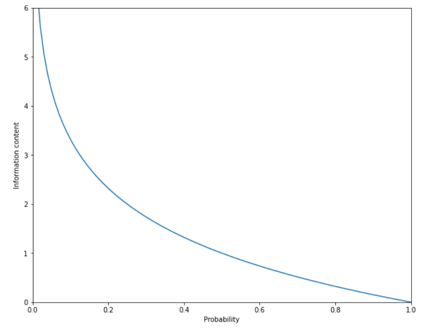
So: forget our old boring discrete random variable $$X$$, and bring in a brand-new continuous random variable that we will call ... $$X$$. How much information do you get from observing $$X$$ land on a particular value $$x$$? You get infinite information, because $$x$$ is a real number with an endless sequence of digits; alternatively, the Shannon information is $$- \log p(x)$$, and the probability of $$X=x$$ is infinitesimally small for a continuous random variable, so the Shannon information is $$-\log 0$$ which is infinite. Umm.

Consider calculating the entropy for a continuous variable, which we will denote $$h(X)$$ to make a difference from the discrete case, and define in the obvious way by replacing sums with integrals: $$$ h(X) = -\int_{-\infty}^\infty f(x) \log f(x) d x $$$ where $$f$$ is the probability density function. If we actually evaluate this integral, we would get a constant term that goes to infinity.

As principled mathematicians, we might be concerned about this. But we can mostly ignore it, especially as the main thing we want is $$I(X;Y)$$, and $$$ I(X;Y) = h(Y) - h(Y|X) = -\int f_Y(y) \log f_Y(y) \mathrm{d}y + \iint f_{X,Y}(x,y) \log f_{Y|X=x}(y) \mathrm{d}x \mathrm{d}y $$$

where mumble mumble the infinities cancel out mumble opposite signs mumble.

Signals

With discrete random variables, we generally had some fairly obvious set of values that they could take. With continuous random variables, we usually deal with an unrestricted range - a radio signal could technically be however low or high. However, step down from abstract maths land, and you realise reality isn't as hopeless as it seems at first. Emitting a radio wave, or making noise, takes some input of energy, and the source has only so much power.

For waves (like radio waves and sound waves), power is proportional to the square of the amplitude of a wave. The variance $$\mathbb{V}(X) = \mathbb{E}[(x-\mathbb{E}[x])^2] = \int f(x) (x - \mathbb{E}[X])^2 \mathrm{d}x$$ of a continuous random variable $$X$$ with probability density function $$f$$ is just the expected squared difference between the value and its mean. Both of these quantities are squaring a difference. It turns out that the power of our source and the variance of the random variable that represents it are proportional.

Our model of a continuous noisy channel is one where there's an input signal $$X$$, a source of noise $$N$$, and an output signal $$Y = X + N$$. As usual, we want to maximise the channel capacity $$C = \max_{p_X} I(X;Y)$$, which is done by maximising $$$ I(X;Y) = h(Y) - h(Y|X). $$$ Because noise is generally the sum of a bunch of small contributing factors in each directions, the noise follows a normal distribution with variance $$\sigma_N^2$$. Because the only source of uncertainty is $$N$$ and this has the same regardless of $$X$$, $$h(Y|X)$$ depends only on $$N$$ and not at all on $$X$$, so the only thing we can affect is $$h(Y)$$.

Therefore, the question of how you maximise channel capacity turns into a question of how to maximise $$h(Y)$$ given that $$Y = X + N$$ with $$N \sim \mathcal{N}(0, \sigma_N^2)$$. If we were working without any power/variance constraints, we'd already know the answer: just make $$X$$ such that $$Y$$ is a uniform distribution (which in this case would mean making $$Y$$ a uniform distribution over all real numbers, something that's clearly a bit wacky). However, we have a constraint on power and therefore the variance of $$X$$.

If we were to do some algebra involving Lagrangian multipliers, we would eventually find that we want the distribution of $$X$$ to be a normal distribution. A key property of normal distributions is that if $$X \sim \mathcal{N}(0, \sigma_X^2)$$ (assume the mean is 0; note you can always shift your scale) and $$N \sim \mathcal{N}(0, \sigma_N^2)$$, then $$X + N \sim \mathcal{N}(0, \sigma_X^2 + \sigma_N^2)$$. Therefore the basic principle between efficiently transmitting information using a continuous signal is that you want to transform your input to follow a normal distribution.

If you do, what do you get? Start with $$$ I(X;Y) = h(Y) - h(Y|X) $$$ and now use the "standard" integral that $$$ \int f(z) \log p(z) \mathrm{d}z = -\frac{1}{2} \log (2 \pi e \sigma^2) $$$ if $$z$$ is drawn from a distribution $$\mathcal{N}(0, \sigma^2)$$, and therefore $$$ \max I(X;Y) = C = \frac{1}{2} \log (2 \pi e (\sigma_X^2 + \sigma_N^2)) - \frac{1}{2} \log (2 \pi e \sigma_N^2) $$$ using the fact that $$h(Y|X) = h(N)$$ since the information content of the noise is all that is unknown about $$Y$$ if we're given $$X$$, and the property of normal distributions mentioned above. We can do some algebra to get the above into the form $$$ C = \frac{1}{2} \log \left(\frac{2 \pi e (\sigma_X^2 + \sigma_N^2)}{2 \pi e \sigma_N^2}\right) \ = \frac{1}{2} \log \left( 1 + \frac{\sigma_X^2}{\sigma_N^2}\right) $$$ The variance is proportional to the power, so this can also be written in terms of power as $$$ C = \frac{1}{2} \log \left( 1 + \frac{S}{N}\right) $$$ if $$S$$ is the power of the signal and $$N$$ is the power of the noise. The units of capacity for the discrete case were bits per symbol; here they're bits per second. A sanity check is that if $$S = 0$$, we transmit $$\frac{1}{2} \log (1) = 0$$ bits per second, which makes sense: if your signal power is 0, it has no effect, and no one is going to hear you.

An interesting consequence here is that increasing signal power only gives you a logarithmic improvement in how much information you can transmit. If you shout twice as loud, you can detect approximately twice as fine-grained peaks and troughs in the amplitude of your voice. However, this helps surprisingly little.

If you want to communicate at a really high capacity, there are better things you can do than shouting very loudly. You can decompose a signal into frequency components using the Fourier transform. If your signal consists of many different frequency levels, you can effectively transmit a different amplitude on each of them at once. The range of frequencies that your signal can span over is called the bandwidth and is denoted $$W$$. If you can make use of multiple frequencies, the capacity equation changes to $$$ C = \frac{W}{2} \log \left(1 + \frac{S}{N}\right) $$$ Therefore if you want to transmit information, transmitting across a broad range of frequencies is much more effective than shouting loudly. There's a metaphor here somewhere.

Information theory 2: source coding

6.9k words, including equations (~36min)

 

In the previous post, we saw the basic information theory model:

If we have no noise in the channel, we don't need channel coding. Therefore the above model simplifies to

and the goal is to minimise $$n$$ - that is, minimise the number of symbols we need to send - without needing to worry about being robust to any errors.

Here's one question to get started: imagine we're working with a compression function $$f_e$$ that acts on length-$$n$$ strings (that is, sequences of symbols) with some arbitrary alphabet size $$A$$ (that is, $$A$$ different types of symbols). is it possible to build an encoding function $$f_e$$ that compresses every possible input? Clearly not; imagine that it took every length-$$n$$ string to a length-$$m$$ string using the same alphabet, with $$m < n$$. Then we'd have $$A^m$$ different available codewords that would need to code for $$A^n > A^m$$ different messages. By the pigeonhole principle, there must be at least one codeword that codes for more than one message. But that means that if we see this codeword, we can't be sure what it codes for, so we can't recover the original with certainty.

Therefore, we have a choice: either:

• do lossy compression, where every message shrinks in size but we can't recover information perfectly; or
• do lossless compression, and hope that more messages shrink in size than expand in size.

This is obvious with lossless compression, but applies to both: if you want to do them well, you generally need a probability model for what your data looks like, or at least something that approximates one.

Terminology

When we talk about a "code", we just mean something that maps messages (the $$Z$$ in the above diagram) to a sequence of symbols. A code is nonsingular if it associates every message with a unique code.

A symbol code is a code where each symbol in the message maps to a codeword, and the code of a message is the concatenation of the codewords of the symbols that it is made of.

A prefix code is a code where no codeword is a prefix of another codeword. They are also called instantaneous codes, because when decoding, you can decode a codeword to a symbol immediately when you reach a point where the some prefix of the code corresponds to a codeword.

Useful basic results in lossless compression

Kraft's inequality

Kraft's inequality states that a prefix code with an alphabet of size $$D$$ and code words of lengths $$l_1, l_2, \ldots, l_n$$ satisfies $$$ \sum_{i=1}^n D^{-l_i} \leq 1, $$$ and conversely that if there is a set of lengths $${l_1, \ldots, l_n}$$ that satisfies the above inequality, there exists a prefix code with those codeword lengths. We will only prove the first direction: that all prefix codes satisfy the above inequality.

Let $$l = \max_i l_i$$ and consider the tree with branching factor $$D$$ and depth $$l$$. This tree has $$D^l$$ nodes on the bottom level. Each codeword $$x_1x_2...x_c$$ is the node in this tree that you get to by choosing the $$d_i$$th branch on the $$i$$th level where $$d_i$$ is the index of symbol $$x_i$$ in the alphabet. Since it must be a prefix code, no node that is a descendant of a node that is a codeword can be a codeword. We can define our "budget " as the $$D^l$$ nodes on the bottom level of the tree, and define the "cost" of each codeword as the number of nodes on the bottom level of the tree that are descendants of the node. The node with length $$l$$ has cost 1, and in general a codeword at level $$l_i$$ has cost $$D^{l - l_i}$$. From this, and the prefix-freeness, we get $$$ \sum_i D^{l - l_i} \leq D^l $$$ which becomes the inequality when you divide both sides by $$D^l$$.

Gibbs' inequality

Gibbs' inequality states that for any two probability distributions $$p$$ and $$q$$, $$$ -\sum_i p_i \log p_i \leq - \sum_i p_i \log q_i $$$ which can be written using the relative entropy $$D$$ (also known as the KL distance/divergence) as $$$ \sum_i p_i \log \frac{p_i}{q_i} = D(p||q) \geq 0. $$$ This can be proved using the log sum inequality. The proof is boring.

Minimum expected length of a symbol code

We want to minimise the expected length of our code $$C$$ for each symbol that $$X$$ might output. The expected length is $$L(C,X) = \sum_i p_i l_i$$. Now one way to think of what a length $$l_i$$ means is using the correspondence between prefix codes and binary trees discussed above. Given the prefix requirement, the higher the level in the tree (and thus the shorter the length of the codeword) the more other options we block out in the tree. Therefore we can think of the collection of lengths we assign to our codewords as specifying a rough probability distribution that assigns probability in proportion to $$2^{-l_i}$$. What we'll do is introduce a variable $$q_i$$ that measures the "implied probability" in this way (note dividing the division by a normalising constant): $$$ q_i = \frac{2^{-l_i}}{\sum_i 2^{-l_i}} = \frac{2^{-l_i}}{z} $$$ where in the 2nd step we've just defined $$z$$ to be the normalising constant. Now $$l_i = - \log zq_i = -\log q_i - \log z$$, so $$$ L(C,X) = \sum_i (-p_i \log q_i) - \log z $$$ Now we can apply Gibbs' inequality to know that $$\sum_i(- p_i \log q_i) \geq \sum_i (-p_i \log p_i)$$ and Kraft's inequality to know that $$\log z = \log \big(\sum_i 2^{-l_i} \big) \leq \log(1)=0$$, so we get $$$ L(C,X) \geq -\sum_i p_i \log p_i = H(X). $$$ Therefore the entropy (with base-2 $$\log$$) of a random variable is a lower bound on the expected length of a codeword (in a 2-symbol alphabet) that represents the outcome of that random variable. (And more generally, entropy with base-$$d$$ logarithms is a lower bound on the length of a codeword for the result in a $$d$$-symbol alphabet.)

Huffman coding

Huffman coding is a very pretty concept.

We saw above that if you're making a random variable for the purpose of gaining the most information possible, you should prepare your random variable to have a uniform probability distribution. This is because entropy is maximised by a uniform distribution, and the entropy of a random variable is the average amount of information you get by observing it.

The reason why, say, encoding English characters as 5-bit strings (A = 00000, B = 00001, ..., Z = 11010, and then use the remaining 6 codes for punctuation or cat emojis or whatever) is not optimal is that some of those 5-bit strings are more likely than others. On a symbol-by-symbol-level, whether the first symbol is a 0 or a 1 is not equiprobable. To get an ideal code, each symbol we send should have equal probability (or as close to equal probability as we can get).

Robert Fano, of Fano's inequality fame, and Claude Shannon, of everything-in-information-theory fame, had tried to find an efficient general coding scheme in the early 1950s. They hadn't succeeded. Fano set it as an alternative to taking the final exam for his information theory class at MIT. David Huffman tried for a while, and had almost given up and started studying instead, when he came up with Huffman coding and quickly proved it to be optimal.

We want the first code symbol (a binary digit) to divide the space of possible message symbols (the English letters, say) in two equally-likely parts, the first two to divide it in four, the third into eight, and so o n. Now some message symbols are going to be more likely than others, so the codes for some symbols have to be longer. We don't want it to be ambiguous when we get to the end of a codeword, so we want a prefix-free code. Prefix-free codes with a size-$$d$$ alphabet can be represented as trees with branching factor $$d$$, where each leaf is one codeword:

Above, we have $$d=2$$ (i..e binary), and six items to code for (a, b, c, d, e, and f), and six code words with lengths of between 1 and 4 characters in the codeword alphabet.

Each codeword is associated with some probability. We can define the weight of a leaf node to be its probability (or just how many times it occurs in the data) and the weight of a non-leaf code to be the sum of the weights of all leaves that are downstream of it in the tree. For an optimal prefix-free code, all we need to do is make sure that each node has children that are as equally balanced in weight as possible.

The best way to achieve this is to work bottom-up. Start without any tree, just a collection of leaf nodes representing the symbols you want codewords for. Then repeatedly build a node uniting the two least-likely parentless nodes in the tree, until the tree has a root.

Above, the numbers next to the non-leaf nodes show the order in which the node was created. This set of weights on the leaf nodes creates the same tree structure as in the previous diagram.

(We could also try to work top-down, creating the tree the root to the leaves rather than from the leaves to the root, but this turns out to give slightly worse results. Also the algorithm for achieving this is less elegant.)

Arithmetic coding

The Huffman code is the best symbol code - that is, a code where every symbol in the message gets associated with a codeword, and the code for the entire message is simply the concatenation of all the codewords of its symbols.

Symbol codes aren't always great, though. Consider encoding the output of a source that has a lot of runs like "aaaaaaaaaahaaaaahahahaaaaa" (a source of such messages might be, for example, a transcription of what a student says right before finals). The Huffman coding for this message is, for example, that "a" maps to a 0, and "h" maps to a 1, and you have achieved a compression of exactly 0%, even though intuitively those long runs of "a"s could be compressed.

One obvious thing you could do is run-length encoding, where long blocks of a character get compressed into a code for the character plus a code for how many times the character is repeated; for example the above might become "10a1h5a1h1a1h1a1h5a". However, this is only a good idea if there are lots of runs, and requires a bunch of complexity (e.g. your alphabet for the codewords must either be something more than binary, or then you need to be able to express things like lengths and counts in binary unambiguously, possibly using a second layer of encoding with a symbol code).

Another problem with Huffman codes is that the code is based on assuming an unchanging probability model across the entire length of the message that is being encoded. This might be a bad assumption if we're encoding, for example, long angry Twitter threads, where the frequency of exclamation marks and capital letters increases as the message continues. We could try to brute-force a solution, such as splitting the message into chunks and fitting a Huffman code separately to each chunk, but that's not very elegant. Remember how elegant Huffman codes feel as a solution to the symbol coding problem? We'd rather not settle for less.

The fundamental idea of arithmetic coding is that we send a number representing where on the cumulative probability distribution of all messages the message we want to send lies. This is a dense statement, so we will unpack it with an example. Let's say our alphabet is $$A = {a, r, t}$$. To establish an ordering, we'll just say we consider the alphabet symbols in alphabetic order. Now let's say our probability distribution for the random variable $$X$$ looks like the diagram on the left; then our cumulative probability distribution looks like the diagram on the right:

One way to specify which of $${a, r, t}$$ we mean is to pick a number $$0 \leq c \leq 1$$, and then look at which range it corresponds to on the $$y$$-axis of the right-hand figure; $$0 \leq c < 0.5$$ implies $$a$$, $$0.5 \leq c < 0.7$$ implies $$r$$, and $$0.7 \leq c < 1$$ implies $$t$$. We don't need to send the leading 0 because it is always present, and for simplicity we'll transmit the following decimals in binary; 0.0 becomes "0", 0.5 becomes "1", 0.25 becomes "01", and 0.875 is "111".

Note that at this point we've almost reinvented is the Huffman code. $$a$$ has the most probability mass and can be represented in one symbol. $$r$$ happens to be representable in one symbol ("1" corresponds to 0.5 which maps to $$r$$) as well even though it has the least probability mass, which is definitely inefficient but not too bad. $$t$$ takes 2: "11".

The real benefit begins when we have multi-character messages. The way we can do it is like this, recursively splitting the number range between 0 and 1 into smaller and smaller chunks:

We see possible numbers encoding "art", "rat", and "tar". Not only that, but we see that all messages we send are infinite in length, as we can just keep going down, adding more and more letters. At first this might seem like a great deal - send one number, get infinite symbols transmitted for free! However, there's a real difference between "art" and "artrat", so we want to be able to know when to stop as well.

A simple answer is that the message also includes some code encoding how many symbols to decode for. A more elegant answer is that we can keep our message as just one number, but extend our alphabet to include an end-of-message token. Note that even with this end-of-message token, it is still true that many characters of the message can be encoded by a single symbol of output, especially if some outcome is much more likely. For example, in the example below we need only one bit ("1", for the number 0.5) to represent the message "aaa" (followed by the end-of-message character):

There are still two ways in which this code is underspecified.

The first is that we need to choose how much of the probability space to assign to our end-of-message token. The optimal value for this clearly depends on how long messages we will be sending.

The second is that even with the end-of-message token, each codeword is still represented by a range of values rather than a single number. Any of these are valid numbers to send, but we want to minimise the length, so therefore we will choose the number in this range that has the shortest binary representation.

Finally, what is our probability model? With the Huffman code, we either assume a probability model based on background information (e.g. we have the set of English characters, and we know the rough probabilities of them by looking at some text corpus that someone else has already compiled), or we fit the probability model based on the message we want to send - if 1/10th of all letters in the message are $$a$$s, we set $$p_a = 0.1$$ when building the tree for our Huffman code, and so on.

With arithmetic coding, we can also assume static probabilities. However, we can also do adaptive arithmetic coding, where we change the probability model as we go. A good way to do this is for our probability model to assume that the probability $$p_x$$ of the symbol $$x$$ after we have already processed text $$T$$ is $$$ p_x = \frac{\text{Count}(x, T) + 1}{\sum_{y \in A} \big(\text{Count}(y, T) + 1\big)}$$$ $$$= \frac{\text{Count}(x, T) + 1}{\sum_{y \in A} \big(\text{Count}(y, T)\big) + |A|} $$$ where $$A$$ is the alphabet, and $$\text{Count}(a, T)$$ simply returns the count of how many times the character $$a$$ occurs in $$T$$. Note that if we didn't have the $$+1$$ in the numerator and in the sum in the denominator, we would assume a probability of zero to anything we haven't seen before, and be unable to encode it.

(We can either say that the end-of-message token is in the alphabet $$A$$, or, more commonly, assign "probabilities" to all $$x$$ using the above formula and some probability $$p_{EOM}$$ to the end of message, and then renormalise by dividing all $$p_x$$ by $$1 + p_{EOM}$$.)

How do we decode this? At the start, the assumed distribution is simply uniform over the alphabet (except maybe for $$p_{EOM}$$). We can decode the first symbol using that distribution, then update the distribution and decode the next, and so on. It's quite elegant.

What isn't elegant is implementing this with standard number systems in most programming languages. For any non-trivial message length, arithmetic coding is going to need very precise floating point numbers, and you can't trust floating point precision very far. You'll need some special system, likely an arbitrary-precision arithmetic library, to actually implement arithmetic coding.

Prefix-free arithmetic coding

The above description of arithmetic coding is not a prefix-free code. We generally want prefix-free codes, in particular because it means we can decode it symbol by symbol as it comes in, rather than having to wait for the entire message to come through. Note also that often in practice it is uncertain whether or not there are more bits coming; consider a patchy internet connection with significant randomness between packet arrival times.

The simple fix for this is that instead of encoding a number as any sequence of binary string that maps onto the right segment of the number line between 0 and 1, you impose an additional requirement on it: whatever binary bits you add onto the number, it is still within the range.

Lempel-Ziv coding

Huffman coding integrated the probability model and the encoding. Arithmetic coding still uses an (at least implicit) probability model to encode, but in a way that makes it possible to update as we encode. Lempel-Ziv encoding, and its various descendants, throw away the entire idea of having any kind of (explicit) probability model. We will look at the original version of this algorithm.

Encoding

Skip all that Huffman coding nonsense of carefully rationing the shorter codewords for the most likely symbols, and simply decide on some codeword length $$d$$ and give every character in the alphabet a codeword of that length. If your alphabet is again $${a, r, t, \text{EOM}}$$ (we'll include the end-of-message character from the start this time), and $$d = 3$$, then the codewords you define are literally as simple as $$$a \mapsto 000 $$$ $$$r \mapsto 001 $$$ $$$t \mapsto 010 $$$ $$$\text{EOM} \mapsto 011$$$ If we used this code, it would be a disaster. We have four symbols in our alphabet, so the maximum entropy of the distribution is $$\log_2 4 = 2$$ bits, and we're spending 3 bits on each symbol. With this encoding, we increase the length by at least 50%. Instead of your compressed file being uploaded in 4 seconds, it now takes 6.

However, we selected $$d=3$$, meaning we have $$2^3 = 8$$ slots for possible codewords of our chosen constant length, and we've only used 4. What we'll do is follow these steps as we scan through our text:

1. Read one symbol past the longest match between the following text and a codeword we've defined. Therefore what we now have is a string $$Cx$$, where we have a code for $$C$$ already of length $$|C|$$, $$x$$ is a single character, and $$Cx$$ is a prefix of the remaining text.
2. Add $$C$$ to the code we're forming, to encode for the first $$|C|$$ characters of the remaining text.
3. If there is space among the $$2^d$$ possible codewords we have available: let $$n$$ be the binary representation of the smallest possible codeword not yet associated with a code, and define $$Cx \mapsto n$$ as a new codeword.

Here is an example of the encoding process, showing the emitted codewords on the left, the original definitions on the top, the new definitions on the right, and the message down the middle:

Decoding

A boring way to decode is to send the codeword list along with your message. The fun way is to reason it out as you go along, based on your knowledge of the above algorithm and a convention that lets you know which order the original symbols were added to the codeword list (say, alphabetically, so you know the three bindings in the top-left). An example of decoding the above message:

Source coding theorem

The source coding theorem is about lossy compression. It is going to tell us that if we can tolerate a probability of error $$\delta$$, and if we're encoding a message consisting of a lot of symbols, unless $$\delta$$ is very close to 0 (lossless compression) or 1 (there is nothing but error), it will take about $$H(X)$$ bits per symbol to encode the message, where $$X$$ is the random variable according to which the symbols in the message have been drawn. Since it means that entropy turns up as a fundamental and surprisingly constant limit when we're trying to compress our information, this further justifies the use of entropy as a measure of information.

We're going to start our attempt to prove the source coding theorem by considering a silly compression scheme. Observe that English has 26 letters, but the bottom 10 (Z, Q, X, J, K, V, B, P, Y, G) are slightly less than 10% of all letters. Why not just drop them? Everthn is still comprehensile without them, and ou can et awa with, for eample, onl 4 inary its per letter rather than 5, since ou're left with ust 16 letters.

Given an alphabet $$A$$ from which our random variable $$X$$ takes values, define the $$\delta$$-sufficient subset $$S_\delta$$ of $$A$$ to be the smallest subset of $$A$$ such that $$P(x \in S_\delta) \geq 1 - \delta$$ for $$x$$ drawn from $$X$$. For example, if $$A$$ is the English alphabet, and $$\delta = 0.1$$, then $$S_\delta$$ is the set of all letters except Z, Q, X, J, K, V, B, P, Y, and G, since the other letters have a combined probability of over $$1 - 0.1 = 0.9$$, and any other subset containing more than $$0.9$$ of the probability mass contains must contain more letters.

Note that $$S_\delta$$ can be formed by adding elements from $$A$$, in descending order of probability, into a set until the sum of probabilities of elements in the set exceeds $$1 - \delta$$.

Next, define the essential bit content of $$X$$, denoted $$H_\delta(X)$$, as $$$ H_\delta(X) = \log 2 |S_\delta|. $$$ In other words, $$H_\delta(X)$$ is the answer to "how many bits of information does it take to point to one element in $$S_\delta$$ (without being able to assume the distribution is anything better than uniform)?". $$H_\delta(X)$$ for $$\text{English alphabet}_{0.1}$$ is 4, because $$\log_2 |{E, T, A, O, I, N, S, H, R, D, L, U, C,M, W, F}| = \log_2 16 = 4$$. It makes sense that this is called "essential bit content".

We can graph $$H_\delta(X)$$ against $$\delta$$ to get a pattern like this:

Where it gets more interesting is when we extend this definition to blocks. Let $$X^n$$ denote the random variable for a sequence of $$n$$ independent identically distributed samples drawn from $$X$$. We keep the same definitions for $$S_\delta$$ and $$H_\delta(X)$$; just remember that now $$S$$ is a subset of $$A^n$$ (where the exponent denotes Cartesian product of a set with itself; i.e. $$A^n$$ is all possible length-$$n$$ strings formed from that alphabet). In other words, we're throwing away the least common length-$$N$$ letter strings first; ZZZZ is out the window first if $$n = 4$$, and so on.

We can plot a similar graph as above, except we're plotting $$\frac{1}{n} H_\delta(x)$$ on the vertical axis to get per-symbol entropy, and there's a horizontal line around the entropy of English letter frequencies:

(Note that the entropy per letter of English drops to only 1.3 if we stop modelling each letter as drawn independently from the others around it, and instead have a model with a perfect understanding of which letters occur together.)

The graph above shows the plot of $$\frac{1}{n}H_\delta(x)$$ against $$\delta$$ for a random variable $$X^n$$ for $$n=1$$ (blue), $$n=2$$) (orange), and $$n=3$$ (green). We see that as $$n$$ increases, the lines become flatter, and the middle portions approach the black line that shows the entropy of the English letter frequency distribution. What you'd see if we continued plotting this graph for larger values of $$n$$ (which might happen for example if you bought me a beefier computer) is that this trend continues; specifically, that there is a value $$n$$ large enough that the graph of $$\frac{1}{n}H_\delta(x)$$ is as close as we want to the black line for the entire length of it, except for an arbitrarily small part near $$\delta = 0$$ and $$\delta = 1$$. Mathematically, we can pick an $$\epsilon > 0$$ such that for $$0 < \delta < 1$$ there exists a positive integer $$n_0$$ such that for all $$n \geq n_0$$, $$$ \left| \frac{1}{n}H_\delta(X^n) - H(X) \right| \leq \epsilon. $$$ Now remember that $$\frac{1}{n}H_\delta(X^n)=\frac{1}{n}\log |S_\delta|$$ was the essential bit content per symbol, or, in other words, the number of bits we need per symbol to represent $$X^n$$ (with error probability $$\delta$$) in the simple coding scheme where we assign an equal-length binary number to each element in $$S_\delta$$ (but hold on: aren't there better codes than ones where all elements in $$S_\delta$$ get an equal-length representation? yes, but we'll see soon that not by very much). Therefore what the above equation is saying is that we can encode $$X^n$$ with error chance $$\delta$$ using a number of bits per symbol that differs from the entropy $$H(X)$$ by only a small constant $$\epsilon$$. This is the source coding theorem. It is a big deal, because we've shown that entropy is related to the number of bits per symbol we need to do encoding in a lossy compression scheme.

(You can get to a similar result with lossless compression schemes where, instead of throwing away the ability to encode all sequences not in $$S_\delta$$ and just accepting the inevitable error, you instead have an encoding scheme where you reserve one bit to indicate whether or not an $$x^n$$ drawn from $$X^n$$ is in $$S_\delta$$, and if it is you encode it like above, and if it isn't you encode it using $$\log |A|^n$$ bits. Then you'll find that the probability of having to do the latter step is small enough that $$\log |A|^n > \log |S_\delta|$$ doesn't matter very much.)

Typical sets

Before going into the proof, it is useful to investigate what sorts of sequences $$x^n$$ we tend to pull out from $$X^n$$ for some $$X$$. The basic observation is that most $$x^n$$ are going to be neither the least probable nor the most probably out of all $$x^n$$. For example, "ZZZZZZZZZZ" would obviously be an unusual set of letters to draw at random if you're selecting them from English letter frequencies. However, so would "EEEEEEEEEE". Yes, this individual sequence is much more likely than "ZZZZZZZZZZ" or any other sequence, but there is only one of them, so getting it would still be surprising. To take another example, the typical sort of result you'd expect from a coin loaded so that $$P(\text{"heads"}) = 0.75$$ isn't runs of only heads, but rather an approximately 3:1 mix of heads and tails.

The distribution of letter counts follows a multinomial distribution (the generalisation of the binomial distribution). Therefore (if you think about what a multinomial distribution is, or if you know that the mean is $$n p_{x_i}$$ for the $$i$$th variable) in $$x^n$$ we'd expect roughly $$np_e$$ of the letter e, $$np_z$$ of the letter z, and so on - and $$np_e \ll n$$ even though $$p_e > p_L$$ for all $$L$$ in the alphabet. Slightly more precisely (if you happen to know this fact), the variance of variable $$x_i$$ is $$np_{x_i}(1-p_{x_i})$$, implying that the standard deviation grows only in proportion to $$\sqrt{n}$$, so for large $$n$$ it is very rare to get an $$x^n$$ with counts of $$x_i$$ that differ wildly from the expected count $$np_{x_i}$$.

Let's define a notion of "typicality" for a sequence $$x^n$$ based on this idea of it being unusual if $$x^n$$ is either a wildly likely or wildly unlikely sequence. The median sequence has $$np_{x_i}$$ of each variable, so has probability $$$ P(x^n) = p_{x_1}^{np_{x_1}}p_{x_2}^{np_{x_2}} \ldots p_{x_n}^{np_{x_n}} $$$ which in turn has a Shannon information content of $$$

• \log P(x^n) = -\sum_i np_{x_i} \log p_{x_i} = n H(X) $$$ Oh look, entropy pops up again. How surprising.

Now we make the following definition: a sequence $$x^n$$ is $$\epsilon$$-typical if its information content per symbol is $$\epsilon$$-close to $$H(X)$$, that is $$$ \left| - \frac{1}{n}\log{P(x^n)} - H(X) \right| <\epsilon. $$$ Define the typical set $$T_{n\epsilon}$$ to be the set of length-$$n$$ sequences (drawn from $$X^n$$) that are $$\epsilon$$-typical.

$$T_{n\epsilon}$$ is a small subset of the set $$A^n$$ of all length-$$n$$ sequences. We can see this through the following reasoning: for any $$x^n \in T_{n\epsilon}$$, $$\frac{1}{n} \log P(x^n) \approx H(X)$$ which implies that $$$ P(x^n) \approx 2^{-nH(X)} $$$ and therefore that there can only be roughly $$2^{nH(X)}$$ such sequences; otherwise their probability would add up to more than 1. In comparison, the number of possible sequences $$|A^n| = 2^{n \log |A|}$$ is significantly larger, since $$\log |A| \leq H(X)$$ for any random variable $$X$$ with alphabet / outcome set $$A$$ (with equality if $$X$$ has a uniform distribution over $$A$$).

The typical set contains most of the probability

Chebyshev's inequality states that $$$ P((X-\mathbb{E}[X])^2 \geq a) \leq \frac{\sigma^2}{a} $$$ where $$\sigma^2$$ is the variance of the random variable $$X$$, and $$a \geq 0$$. It is proved here (search for "Chebyshev").

Earlier we defined the $$\epsilon$$-typical set as $$$ T_{n\epsilon} = \left\{ x^n \in A^n \,\text{ such that } \, \left| -\frac{1}{n}\log P(X^n) - H(X) \right| < \epsilon \right\}. $$$ Note that $$$ \mathbb{E}\left[-\frac{1}{n}\log P(X^n)\right] = -\frac{1}{n} \sum \log P(X_i)$$$ $$$ = -\mathbb{E}[\log P(X_i)]$$$ $$$ = H(X_i) = H(X) $$$ by using independence of the $$X_i$$ making up $$X^n$$ in the first step, the law of large numbers ($$\lim_{n \to \infty} \frac{1}{n} \sum_i X_i = \mathbb{E}[X]$$) in the second, and the fact that all $$X_i$$ are independent draws of the same random variable $$X$$ in the third.

Therefore, we can now rewrite the typical set definition equivalently as $$$ T_{n\epsilon} = \left\{ x^n \in A^n \,\text{ such that } \, \left( -\frac{1}{n}\log P(x^n) - H(X) \right)^2 < \epsilon^2 \right\}$$$ $$$= \left\{ x^n \in A^n \,\text{ such that } \, \left( Y - \mathbb{E}[Y] \right)^2 < \epsilon^2 \right\} $$$ for $$Y = -\frac{1}{n} \log P(X^n)$$, which is in the right form to apply Chebyshev's inequality to get a probability of belonging to this set, except for the fact that the sign is the wrong way around. Very well - we'll instead consider the set of sequences $$\bar{T}_{n\epsilon} = A^n - T_{n\epsilon}$$ (i.e. all length-$$n$$ sequences that are not typical) instead, which can be defined as $$$ \bar{T}_{n \epsilon} = \left\{ x^n \in A^n \,\text{ such that } \, (Y - \mathbb{E}[Y])^2 \geq \epsilon^2 \right\} $$$ and use Chebyshev's inequality to conclude that $$$ P((Y - \mathbb{E}[Y])^2 \geq \epsilon^2) \leq \frac{\sigma_Y^2}{\epsilon^2} $$$ where $$\sigma_Y^2$$ is the variance of $$Y= -\frac{1}{n} \log P(X^n)$$. This is exciting - we have a bound on the probability that a sequence is not in the typical set - but we want to link this probability to $$n$$ somehow. Let $$Z = -\log P(X)$$, and note that $$Y$$ can be written as the average of many draws from $$Z$$. Therefore $$$ \mathbb{E}[Z] = -\frac{1}{n} \sum_i \log P(X) = -\frac{1}{n} \log P(X^n) = \mathbb{E}[Y] $$$ and since $$Y = \frac{1}{n} \sum_i Z_i$$, the variance of $$Y$$, $$\sigma_Y^2$$, is equal to $$\frac{1}{n} \sigma_Z^2$$ (a basic law of how variance works that is often used in statistics). We can substitute this into the expression above to get $$$ P((Y-\mathbb{E}[Y])^2 \geq \epsilon^2) \leq \frac{\sigma_Z^2}{n\epsilon^2}. $$$ The probability on the left-hand side is identical to $$P((-\frac{1}{n} \log P(X^n) - H(X) )^2 \geq \epsilon^2)$$, which is the probability of the condition that $$X^n$$ is not in the $$\epsilon$$-typical set $$T_{n\epsilon}$$, which gives us our grand result $$$ P(X^n \in T_{n\epsilon}) \ge 1 - \frac{\sigma_Z^2}{n\epsilon^2}. $$$ $$\sigma_Z^2$$ is the variance of $$\log P(X^n)$$; it depends on the particulars of the distribution and is probably hell to calculate. However, what we care about is that if we just crank up $$n$$, we can make this probability as close to 1 as we like, regardless of what $$\sigma_Z^2$$ is, and regardless of what we set as $$\epsilon$$ (the parameter for how wide the probability range for the typical set).

The key idea is this: asymptotically, as $$n \to \infty$$, more and more of the probability mass of possible length-$$n$$ sequences is concentrated among those that have a probability of between $$2^{-n(H(X)+\epsilon)}$$ and $$2^{-n(H(x) - \epsilon)}$$, regardless of what (positive real) $$\epsilon$$ you set. This is known as the "asymptotic equipartition property" (it might be more appropriate to call it an "asymptotic approximately-equally-partitioning property" because it's not really an "equipartition", since depending on $$\epsilon$$ these can be very different probabilities, but apparently that was too much of a mouthful even for the mathematicians).

Finishing the proof

As a reminder of where we are: we stated without proof $$$ \left| \frac{1}{n}H_\delta(X^n) - H(X) \right| < \epsilon. $$$ and noted that this is an interesting result that also gives meaning to entropy, since we see that it's related to how many bits it takes for a naive coding scheme to express $$X^n$$ (with error probability $$\delta$$).

Then we went on to talk about typical sets, and ended up finding that the probability that an $$x^n$$ drawn from $$X^n$$ lies in the set $$$ T_{n \epsilon} =\left\{ x^n \in A^n \,\text{ such that } \, \left| -\frac{1}{n}\log P(X^n) - H(X) \right| < \epsilon \right\}. $$$ approaches 1 as $$n \to \infty$$, despite the fact that $$T_{n\epsilon}$$ has only approximately $$2^{nH(X)}$$ members, which, for distributions of $$X$$ that are not very close to the uniform distribution over the alphabet $$A$$, is a small fraction of the $$2^{n \log |A|}$$ possible length-$$n$$ sequences.

Remember that $$H_\delta(X^n) = \log |S_\delta|$$, and $$S_\delta$$ was the smallest subset of $$A^n$$ such that it contains sequences whose probability sums to at least $$1 - \delta$$. This is a bit like the typical set $$T_{n\epsilon}$$, which also contains sequences making up most of the probability mass. Note that $$T_{n\epsilon}$$ is less efficient; $$S_\delta$$ optimally contains all sequences with probability greater than some threshold, whereas $$T_{n\epsilon}$$ generally omits the highest-probability sequences (settling instead for sequences of the same probability as most sequences that are drawn from $$X^n$$). Therefore $$$ H_\delta(X^n) \leq \log |T_{n\epsilon}| $$$ for an $$n$$ that depends on what $$\delta$$ and $$\epsilon$$ we want. Now we can get an upper bound on $$H_\delta(X^n)$$ if we can upper-bound $$|T_{n\epsilon}|$$. Looking at the definition, we see that the probability of a sequence $$X^n$$ must obey $$$ 2^{n(H(X) - \epsilon)} < P(X^n) < 2^{n(H(X) + \epsilon)}. $$$ $$T_{n\epsilon}$$ has the largest number of elements if all elements have the lowest possible probability $$p$$, and if that is the case it has at most $$1/p$$ of such lowest-probability elements since the probabilities cannot add to more than one, which implies $$|T_{n\epsilon}| < 2^{n(H(x)+\epsilon)}$$. Therefore $$$ H_\delta(X^n) \leq \log |T_{n\epsilon}| < \log(2^{n(H(X)+e)}) = n(H(X) + \epsilon) $$$ and we have a bound $$$ H_\delta(X^n) < n(H(X) + \epsilon). $$$ If we can now also find the bound $$n(H(X) + \epsilon) < H_\delta(X^n)$$, we've shown $$|\frac{1}{n} H_\delta(X^n) - H(X)| < \epsilon$$ and we're done. The proof of this bound is a proof by contradiction. Imagine that there is an $$S'$$ such that $$$ \frac{1}{n} \log |S'| \leq H - \epsilon $$$ but also $$$ P(X^n \in S') \geq 1 - \delta. $$$ We want to show that $$P(X^n \in S')$$ can't actually be that large. For the other bound, we used our typical set successfully, so why not use it again? Specifically, write $$$ P(X^n \in S') = P(X^n \in S' \cap T_{n\varepsilon}) + P(X^n \in S' \cap \bar{T}_{n\varepsilon}) $$$ where $$\bar{T}_{n\varepsilon}$$ is again $$A^n - T_{n\varepsilon}$$, and noting that our constant $$\varepsilon$$ for $$T$$, is not the same as our constant $$\epsilon$$ in the bound. We want to set an upper bound on this probability; for that to hold, we need to make the terms on the right-hand side as large as possible. For the term, this is if $$S' \cap T_{n\varepsilon}$$ is as large as it can be based on the bound on $$|S'|$$, i.e. $$2^{n(H(X)-\epsilon)}$$, and each term in it has the maximum probability $$2^{-n(H(X)-\varepsilon)}$$ of terms in $$T_{n\varepsilon}$$. For the second term, this is if $$S' \cap \bar{T}_{n \epsilon}$$ is restricted only by $$P(X^n \in \bar{T}_{n\varepsilon}) \leq \frac{\sigma^2}{n\epsilon^2}$$, which we showed above. (Note that you can't have both of these conditions holding at once, but this does not matter since we only want to show a non-strict inequality.) Therefore we get $$$ P(X^n \in S') \leq 2^{n(H(X) - \epsilon)} 2^{-n(H(X)+\varepsilon)} + \frac{\sigma^2}{n\epsilon^2} \ = 2^{-n(\epsilon + \varepsilon)} + \frac{\sigma^2}{n\epsilon^2} $$$ and we see that since $$\epsilon, \varepsilon > 0$$, and as we're dealing with the case where $$n \to \infty$$, this probability is going to go to zero in the limit. But we had assumed $$P(X^n \in S') \geq 1 - \delta$$ - so we have a contradiction unless we don't assume that, which means $$$ n(H(X) - \epsilon) < H_\delta(X^n). $$$ Combining this with the previous bound, we've now shown $$$ H(X) - \epsilon < \frac{1}{n} H_\delta(X^n) < H(X) + \epsilon $$$ which is the same as $$$ \left|\frac{1}{n}H_\delta(X) - H(X)\right| < \epsilon $$$ which is the source coding theorem that we wanted to prove.

Information theory 1

5044 words, including equations (~30min)

This is the first in a series of posts about information theory. A solid understanding of basic probability (random variables, probability distributions, etc.) is assumed. This post covers:

• what information and entropy are, both intuitively and axiomatically
• (briefly) the relation of information-theoretic entropy to entropy in physics
• conditional entropy
• joint entropy
• KL distance (also known as relative entropy)
• mutual information
• some results involving the above quantities
• the point of source coding and channel coding

Future posts cover source coding and channel coding in detail.

What is information?

How much information is there in the number 14? What about the word "information"? Or this blog post? These don't seem like questions with exact answers.

Imagine you already know that someone has drawn a number between 0 and 15 from a hat. Then you're told that the number is 14. How much additional information have you learned? A first guess at a definition for information might be that it's the number of questions you need to ask to become certain about an answer. We don't want arbitrary questions though; "what is the number?" is very different from "is the number zero?". So let's say that it has to be a yes-no question.

You can represent a number within some specific range as a series of yes-no questions by writing it out in base-2. In base-2, 14 is 1110. Four questions suffice: "is the leftmost base-2 digit a 0?", etc. The number of base-$$B$$ digits required to represent a number $$n$$ is $$\lceil\log_B n\rceil$$, where $$\lceil x \rceil$$ means the smallest integer greater than or equal to $$x$$ (i.e., rounding up). Now maybe there should be some sense in which we can allow pointing at a number in the range 0 to 16 to have a bit more information than pointing at a number from 0 to 15, even though we can't literally ask 4.09 yes-no questions. So we might try to define our information measure as $$\log n$$ (in whatever base because changing which base we're doing logs in would only change the answer by a constant factor anyways, but let's just say it's base-2 to maintain the correspondence to yes-no questions), where $$n$$ is the number of outcomes that the thing we now know was selected from.

Now let's say there's a shoe box we've picked up from a store. There are a gazillion things that could be inside the box, so $$n$$ is something huge. However, it seems that if we open the box and find a new pair of sneakers, we are less surprised than if we open the box and find the Shroud of Turin. We'd like to make some types of contain quantitatively more information than others.

The standard sort of thing you do in this kind of situation is that you bring in probabilities. With drawing a number out of a hat, we have a uniform distribution where the probability for each outcome is $$p = 1/ n$$. So therefore we might as well have written that information content is equivalent to $$\log \frac{1}{p}$$, and gotten the same answer in that question. Since presumably the probability of your average shoe box containing sneakers is higher than the probability of it containing the Shroud of Turin, with this revised definition we now sensibly get that the latter gives us more information (because $$\log \frac{1}{p}$$ is a decreasing function of $$p$$). Note also that $$\log \frac{1}{p}$$ is the same as $$- \log p$$; we will usually use the latter form. This is called the Shannon information. To be precise:

The (Shannon) information content of seeing a random variable $$X$$ take a value $$x$$ is $$$-\log p_x$$$ where $$p_x$$ is the probability that $$X$$ takes value $$x$$.

We can see the behaviour of the information content of an event as a function of its probability here:

Axiomatic definition

The above derivation was so hand-wavy that it wasn't even close to being a derivation.

When discovering/inventing the concept of Shannon information, Shannon started from the idea that the information contained in seeing an event is a function of that event's probability (and nothing else). Then he required three further axioms to hold for this function:

• If the probability of an outcome is 1, it contains no information. This makes sense - if you already know something with certainty, then you can't get more information by seeing it again.
• The information contained in an event is a decreasing function of its probability of happening. Again, this makes sense: seeing something you think is very unlikely is more informative than seeing something you were pretty certain was already going to happen.
• The information contained in seeing two independent events is the sum of the information of seeing them separately. We don't want to have to apply some obscure maths magic to figure out how much information we got in total from seeing one dice roll and then another other.

The last one is the big hint. The probability of seeing random variable (RV) $$X$$ take value $$x$$ and RV $$Y$$ take value $$y$$ is $$p_x p_y$$ if $$X$$ and $$Y$$ are independent. We want a function, call it $$f$$, such that $$f(p_x p_y) = f(p_x) + f(p_y)$$. This is the most important property of logarithms. You can do some more maths to really demonstrate that is the logarithms with some base are the only function that fit this definition, or you can just guess that it's a $$\log$$ and move on. We'll do the latter.

Entropy

Entropy is the flashy term that comes up in everything from chemistry to .zip files to the fundamental fact that we're all going to die. It is often introduced as something like "[mumble mumble] a measure of information [mumble mumble]".

It is important to distinguish between information and entropy. Information is a function of an outcome (of a random variable), for example the outcome of an experiment. Entropy is a function of a random variable, for example an experiment before you see the outcome. Specifically,

The entropy $$H(X)$$ is the expected information gain from a random variable $$X$$: $$$ H(X) = \underset{x_i \sim X}{\mathbb{E}}\Big[-\log P(X=x_i)\Big] \ = -\sum_i p_{x_i} \log p_{x_i} $$$ ($$\underset{x_i \sim X}{\mathbb{E}}$$ means the expected value when value $$x_i$$ is drawn from the distribution of RV $$X$$. $$P(X=x_i)$$, alternatively denoted $$p_{x_i}$$ when $$X$$ is clear from context, is the probability of $$X$$ taking value $$x_i$$.)

(Why is entropy denoted with an $$H$$? I don't know. Just be thankful it wasn't a random Greek letter.)

Imagine you're guessing a number between 0 and 15 inclusive, and the current state of your beliefs is that it is as likely to be any of these numbers. You ask "is the number 9?". If the answer is yes, you've gained $$-\log_2 \frac{1}{16} = \log_2 16 = 4$$ bits of information. If the answer is no, you've gained $$-\log_2 \frac{15}{16} = \log_2 16 - \log_2 15 = 0.093$$ bits of information. The probability of the first outcome is 1/16 and the probability of the second is 15/16, so the entropy is $$\frac{15}{16} \times 4 + \frac{1}{16} \times 0.093 = 0.337$$ bits.

In contrast, if you ask "is the number smaller than 8?", you always get $$-\log_2 \frac{8}{16} = \log_2{2} = 1$$ bit of information, and therefore the entropy of the question is 1 bit.

Since entropy is expected information gain, whenever you prepare a random variable for the purpose of getting information by observing its value, you want to maximise its entropy.

The closer a probability distribution is to a uniform distribution, the higher its entropy. The maximum entropy of a distribution with $$n$$ possible outcomes is the entropy of the uniform distribution $$U_n$$, which is $$$ H(U_n) = -\sum_i p_{u_i} \log p_{u_i} = -\sum_i \frac{1}{n} \log \frac{1}{n} \ = -\log \frac{1}{n} = \log n $$$ (This can be proved easily once we introduce some additional concepts.)

A general and very helpful principle to remember is that RVs with uniform distributions are most informative.

The above definition of entropy is sometimes called Shannon entropy, to distinguish it from the older but weaker concept of entropy in physics.

Entropy in physics

The physicists' definition of entropy is a constant times the logarithm of the number of possible states that correspond to the observable macroscopic characteristics of a thermodynamic system: $$$ S=k_B \ln W $$$ where $$k_B$$ is the Boltzmann constant, $$\ln$$ is used instead of $$\log_2$$ because physics, and $$W$$ is the number of microstates. (Why do physicists denote entropy with the letter $$S$$? I don't know. Just be glad it wasn't a random Hebrew letter.)

In plain language: it is proportional to the Shannon entropy of finding out what is the exact configuration of bouncing atoms of the hot/cold/whatever box you're looking, out of all the ways the atoms could be bouncing inside that box given that the box is hot/cold/whatever, assuming that all those ways are equally likely. It is less general than the information theoretic entropy in the sense that it assumes a uniform distribution.

Entropy, either the Shannon or the physics version, seems abstract; random variables, numbers of microstates, what? However, $$S$$ as defined above has very real physical consequences. There's an important thermodynamics equation relating a change in entropy $$\delta S$$, a change in heat energy $$\delta Q$$, and temperature $$T$$ for a reversible process with the equation $$T\delta S = \delta Q$$, which sets a lower bound on how much energy you need to discover information (i.e., reduce the number of microstates that might be behind the macrostate you observe). Getting one bit of information means that $$\delta S$$ is $$k_B \ln 2$$ (from the definition of $$S$$), so at temperature $$T$$ kelvins we need $$k_B T \ln 2 \approx 9.6 \times 10^{-24} \times T$$ joules. This prevents arbitrarily efficient computers, and saves us from problems like Maxwell's demon. (Maxwell's demon is a thought experiment in physics: couldn't you violate the principle of increasing entropy (a physics thing) by building a box with a wall cutting it in half with a "demon" (some device) that lets slow particles pass left-to-right only and fast particles right-to-left, thus separating particles by temperature and reducing the number of microstates corresponding to the configuration of atoms inside the box? No, because the demon needs to expend energy to get information.)

Finally, is there an information-theoretic analogue of the second law of thermodynamics, which states that the entropy of a system always increases? You have to make some assumptions, but you can get to something like it, which I will sketch out in very rough detail and without explaining the terms (see Chapter 4 of Elements of Information Theory for the details). Imagine you have a probability distribution on the state space of a Markov chain. Now it is possible to prove that given any two such probability distributions, the distance between them (as measured using relative entropy; see below) is non-increasing. Now assume it also happens to be the case that the stationary distribution of the Markov chain is uniform (the stationary distribution is the probability distribution over states such that if every state sends out its probability mass according to the transition probabilities, you get back to the same distribution). We can consider an arbitrary probability distribution over the states, and compare it to the unchanging uniform one, and use the result that the distance between them is non-increasing to deduce that an arbitrary probability distribution will tend towards the uniform (= maximal entropy) one.

Reportedly, von Neumann (a polymath whose name appears in any mid-1900s mathsy thing) advised Shannon thus:

"You should call [your concept] entropy, for two reasons. In the first place your uncertainty function has been used in statistical mechanics under that name, so it already has a name. In the second place, and more important, nobody knows what entropy really is, so in a debate you will always have the advantage."

Intuition

We've snuck in the assumption that all information comes in the form of:

1. You first have some quantitative uncertainty over a known set of possible outcomes, which you specify in terms of a random variable $$X$$.
2. You find out the value that $$X$$ has taken.

There's a clear random variable if you're pulling numbers out of a hat: the possible values of $$X$$ are the numbers written on the pieces of paper in the hat, and they all have equal probability. But where is the random variable when the piece of information you get is, say, the definition of information? (I don't mean here the literal characters on the screen - that's a more boring question - but instead the knowledge about information theory that is now (hopefully) in your brain). The answer would have to be something like "the random variable representing all possible definitions of information" (with a probability distribution that is, for example, skewed towards definitions that include a $$\log$$ somewhere because you remember seeing that before).

This is a bit tricky to think about, but we see that even in this kind of weird case you can specify some kind of set and probabilities over that set. Fundamentally, knowledge (or its lack) is about having a probability distribution over states. Perfect knowledge means you have probability $$1.00$$ on exactly one state of how something could be. If you're very uncertain, you have a huge probability distribution over an unimaginably large set of states (for example, all possible concepts that might be a definition of information). If you've literally seen nothing, then you're forced to rely on some guess for the prior distribution over states, like all those pesky Bayesian statisticians keep saying.

More quantities

Conditional entropy

Entropy is a function of the probability distribution of a random variable. We want to be able to calculate the entropies of the random variables we encounter.

A common combination of random variables we see is $$X$$ given $$Y$$, written $$X | Y$$. The definition is $$$ P(X = x \, |\, Y = y) = \frac{P(X = x \,\land\, Y = y)}{P(Y=y)}. $$$ It is a common mistake to think that $$H(X|Y) = -\sum_i P(X = x_i | Y = y) \log P(X = x_i | Y = y)$$. What is it then? Let's just do the algebra: $$$ H(X|Y) = -\underset{x \sim X|Y, y \sim Y}{\mathbb{E}} \big( \log P(X=x|Y=y) \big) $$$ from the definition of the entropy as the expectation of the Shannon information content, and then by algebra: $$$ H(X|Y) = -\underset{x \sim X|Y, y \sim Y}{\mathbb{E}} \big[ \log P(X=x|Y=y) \big]$$$ $$$ = -\sum_{y \in \mathcal{Y}} P(Y=y) \sum_{x \in \mathcal{X}} P(X=x | Y=y) \log P(X=x \,|\, Y = Y)$$$ $$$ = -\sum_{y \in \mathcal{Y}, \, x \in \mathcal{X}}P(X=x\,\land\, Y = y) \log P(X=x \,|\, Y = Y) $$$ where $$\mathcal{X}$$ and $$\mathcal{Y}$$ are simply the sets of possible values of $$X$$ and $$Y$$ respectively. In a trick beloved of bloggers everywhere tired of writing up equations as $$\LaTeX$$, the above is often abbreviated $$$ \sum_{y \in \mathcal{Y}, \, x \in \mathcal{X}} p(x,y) \log p(x|y) $$$ where we use $$p$$ as a generic notation for "probability of whatever; random variables left implicit".

The conditional entropy $$X|Y$$ for a random variable $$X$$ given the value of another random variable $$Y$$, is written $$H(X|Y)$$ and defined as $$$ H(X|Y) = - \sum_{y \in \mathcal{Y}, \, x \in \mathcal{X}} p(x,y) \log p(x|y) $$$ which is lazier notation for $$$ -\sum_{y \in \mathcal{Y}, \, x \in \mathcal{X}}P(X=x\,\land\, Y = y) \log P(X=x \,|\, Y = Y). $$$ and also equal to $$$ -\sum_{y \in \mathcal{Y}, \, x \in \mathcal{X}} p(x,y) \log \frac{p(x, y)}{p(y)} $$$ It is most definitely not equal to $$\sum_{y \in \mathcal{Y}, \, x \in \mathcal{X}} p(x | y) \log p(x | y)$$.

Conditional entropy is a measure of how much information we expect to get from a random variable assuming we've already seen another one. If the RVs $$X$$ and $$Y$$ are independent, the answer is that $$H(X|Y) = H(X)$$. If the value of $$Y$$ implies a value of $$X$$ (e.g. "percentage of sales in the US" implies "percentage of sales outside the US"), then $$H(X|Y) = 0$$, since we can work out what $$X$$ is from seeing what $$Y$$ is.

Joint entropy

Now if $$H(X|Y)$$ is how much expected surprise there is left in $$X$$ after you've seen $$Y$$, then $$H(X|Y) + H(Y)$$ would sensibly be the total expected surprise in the combination of $$X$$ and $$Y$$. We write $$H(X,Y)$$ for this combination. If we do the algebra, we see that $$$ H(X,Y) = H(X|Y) + H(Y) $$$ $$$ = -\sum_{y \in \mathcal{Y}, \, x \in \mathcal{X}} p(x,y) \log \frac{p(x, y)}{p(y)} - \sum_{y \in \mathcal{Y}} p(y) \log p(y) $$$ $$$= -\left(\sum_{y \in \mathcal{Y}, \, x \in \mathcal{X}} p(x,y) \log p(x, y)\right) + \left( \sum_{y \in \mathcal{Y}, \,x\in \mathcal{X}} p(x,y) \log p(y)\right) -\left( \sum_{y \in \mathcal{Y}} p(y) \log p(y)\ \right) $$$ $$$= -\left(\sum_{y \in \mathcal{Y}, \, x \in \mathcal{X}} p(x,y) \log p(x, y)\right)$$$ = H(Z) $$$ if $$Z$$ is the random variable formed of the pair $$(X, Y)$$ drawn from the joint distribution over $$X$$ and $$Y$$.

Kullback-Leibler divergence, AKA relative entropy

"Kullback-Leibler divergence" is a bit of a mouthful. It is also called KL divergence, KL distance, or relative entropy. Intuitively, it is a measure of the distance between two probability distributions. For probability distributions represented by functions $$p$$ and $$q$$ over the same set $$\mathcal{X}$$, it is defined as $$$ D(p\,||\,q) = \sum_{x \in \mathcal{X}} p(x) \log \left(\frac{p(x)}{q(x)}\right). $$$ It's not a very good distance function; the only property of a distance function it meets is that it's non-negative. It's not symmetric (i.e. $$D(p \,||\, q) \ne D(q \,||\, p)$$) as you can see from the definition (especially considering how it breaks when $$q(x) = 0$$ but not if $$p(x) = 0$$). However, it has a number of cool interpretations, including how many bits you expect to lose on average if you build a code assuming a probability distribution $$q$$ when it's actually $$p$$, and how many bits of information you get in a Bayesian update from distribution $$q$$ to distribution $$p$$. It is also a common loss function in machine learning. The first argument $$p$$ is generally some better or true model, and we want to know how far away $$q$$ is from it.

Why the uniform distribution maximises entropy

The KL divergence gives us a nice way of proving that the uniform distribution maximises entropy. Consider the KL divergence of an arbitrary probability distribution $$p$$ from the uniform probability distribution $$u$$: $$$ D(p \,||\, u ) = \sum_{x \in \mathcal{X}} p(x) \log \left(\frac{p(x)}{q(x)}\right) $$$ $$$= \sum_{x \in \mathcal{X}} \big( p(x) \log p(x)\big) - \sum_{x \in \mathcal{X}} \big(p(x) \log q(x) \big) $$$ $$$= -H(X) - \sum_{x \in \mathcal{X}} p(x) \log \frac{1}{|\mathcal{X}|} $$$ $$$= H(X) - H(U) $$$ where $$\mathcal{X}$$ is the set of values over which $$p$$ and $$u$$ have non-zero values, $$X$$ is a random variable distributed according to $$p$$, and $$U$$ is a random variable distributed according to $$u$$ (i.e. uniformly). This is the same thing as $$$ H(X) = H(U) + D(p \,||\,u) $$$ which implies that we can write the entropy of a random variable as the entropy of a uniform random variable over a set of the same size, plus the KL distance between the distribution of $$X$$ and the distribution of the uniform random variable. Also, since all three quantities in the above equation are guaranteed to be non-negative, this implies that $$$ H(X) \leq H(U) $$$ and therefore that the uniform random variable has higher entropy than any other random variable over the same number of outcomes.

Mutual information

Earlier, we saw that $$H(X, Y) = H(X|Y) + H(Y) = H(X) + H(Y|X)$$. As a picture:

There's an overlapping region, representing the information you get no matter which of $$X$$ or $$Y$$ you look at. We call this the mutual information, a refreshingly sensible name, and denote it $$I(X;Y)$$, somewhat less sensibly. One way to find it is $$$ I(X;Y) = H(X,Y) - H(X|Y) - H(Y|X)$$$ $$$= - \sum_{x,y} p(x,y) \log p(x,y) \,+\, \sum_{x,y} p(x,y) \log \frac{p(x,y)}{p(y)} \,+\, \sum_{x,y} p(x,y) \log \frac{p(x,y)}{p(x)}$$$ $$$= \sum_{x,y} p(x,y) \big( \log p(x,y) - \log p(x) - \log p(y) \big)$$$ $$$= \sum_{x,y} p(x,y) \log \frac{p(x,y)}{p(x)p(y)}. $$$ Does this look familiar? Recall the definition $$$ D(p\,||\,q) = \sum_{x \in \mathcal{X}} p(x) \log \left(\frac{p(x)}{q(x)}\right). $$$ What we see is that $$$ I(X;Y) = D(p(x, y) \, || \, p(x) p(y)), $$$ or in other words that the mutual information between $$X$$ and $$Y$$ is the "distance" (as measured by KL divergence) between the probability distributions $$p(x,y)$$ - the joint distribution between $$X$$ and $$Y$$ - and $$p(x) p(y)$$, the joint distribution that $$X$$ and $$Y$$ would have if $$x$$ and $$y$$ were drawn independently.

If $$X$$ and $$Y$$ are independent, then these are the same distribution, and their KL divergence is 0.

If the value of $$Y$$ can be determined from the value of $$X$$, then the joint probability distribution of $$X$$ and $$Y$$ is a table where for every $$x$$, there is only one $$y$$ such that $$p(x,y) > 0$$ (otherwise, there would be a value $$x$$ such that there is uncertainty about $$Y$$). Let the function mapping an $$x$$ to the singular $$y$$ such that $$p(x,y) > 0$$ be $$f$$. Then $$$ I(X;Y) = \sum_{x,y} p(x,y) \log \frac{p(x,y)}{p(x)p(y)}$$$ $$$= \sum_y p(y) \sum_{x | f(x) = y} p(x|y) \log \frac{p(x, f(x))}{p(x)p(y)}. $$$ Now $$p(x, f(x)) = p(x)$$, because there is no $$y \ne f(x)$$ such that $$p(x, y) \ne 0$$. Therefore we get that the above is equal to $$$ \sum_y p(y) \sum_{x | f(x) = y} p(x|y) \log \frac{p(x)}{p(x)p(y)}\ = - \sum_y p(y) \sum_{x | f(x) = y} p(x|y) \log p(y), $$$ and since $$\log p(y)$$ does not depend on $$x$$, we can sum out the probability distribution to get $$$ -\sum_y p(y) \log p(y) = H(Y). $$$ In other words, if $$Y$$ can be determined from $$X$$, then the expected information that $$X$$ gives about $$Y$$ is the same as the expected information given by $$Y$$.

We can graphically represent the relations between $$H(X)$$, $$H(Y)$$, $$H(X|Y)$$, $$H(Y|X)$$, $$H(X,Y)$$, and $$I(X;Y)$$ like this:

Having this image in your head is the single most valuable thing you can do to improve your ability to follow information theoretic maths. Just to spell it out, here are some of the results you can read out from it: $$$H(X,Y) = H(X) + H(Y|X) $$$ $$$H(X,Y) = H(X|Y) + H(Y) $$$ $$$H(X,Y) = H(X|Y) + I(X;Y) + H(Y|X) $$$ $$$H(X,Y) = H(X) + H(Y) - I(X;Y) $$$ $$$H(X) = I(X;Y) + H(Y|X)$$$ This diagram is also sometimes drawn with Venn diagrams:

Data processing inequality

A Markov chain is a series of random variables such that the $$(n+1)$$th is only directly influenced by the $$n$$th. If $$X \to Y \to Z$$ is a Markov chain, it means that all effects $$X$$ has on $$Z$$ are through $$Y$$.

The data processing inequality states that if $$X \to Y \to Z$$ is a Markov chain, then $$$ I(X; Y) \geq I(X; Z). $$$ This should be pretty intuitive, since the mutual information $$I(X;Y)$$ between $$X$$ and $$Y$$, which have a direct causal link between them, shouldn't be higher than that between $$X$$ and the more-distant $$Z$$, which $$X$$ can only influence through $$Y$$.

A special case is the Markov chain $$X \to Y \to f(Y)$$, where $$X$$ is, say, what happened in an abandoned parking lot at 3am, $$Y$$ is the security camera footage, and $$f$$ is some image enhancing process (more generally: any deterministic function of the data $$Y$$). The data processing inequality tells us that $$$ I(X; Y) \geq I(X; f(Y)). $$$ In essence, this means that any function you try to apply to some data $$Y$$ you have about some event $$X$$ cannot increase the information about the event that is available. Any enhancing function can only make it easier to spot some information about the event that is already present in the data you have about it (and the function might very plausibly destroy some). If all you have are four pixels, no amount of image enhancement wizardry will let you figure out the perpetrator's eye colour.

The proof (for the general case of $$X \to Y \to Z$$) goes like this: consider $$I(X; Y,Z)$$ (that is, the mutual information between knowing $$X$$ and knowing both $$Y$$ and $$Z$$). Now consider the different values in Venn diagram form:

$$I(X; Y, Z)$$ corresponds to all areas within the circle representing $$X$$ that are also within at least one of the circle for $$Y$$ or $$Z$$. If we knew both $$Y$$ and $$Z$$, this "bite" is how much would be taken out of the uncertainty $$H(X)$$ of $$X$$.

We see that the red lined area is $$I(X; Y|Z)$$ (the information shared between $$X$$ and the part of $$Y$$ that remains unknown if you know $$Z$$), and likewise the green hatched area is $$I(X; Y; Z)$$ and the blue dotted area is $$I(X;Z|Y)$$. Since the red-lined and green-hatched areas together are $$I(X;Y)$$, and the green-hatched and blue-dotted areas together are $$I(X;Z)$$, we can write both $$$ I(X; \,Y,Z) = I(X;\,Y) + I(X;\,Z|Y)$$$ $$$I(X; \,Y,Z) = I(X;\,Z) + I(X;\,Y|Z) $$$ But hold on - $$I(X;Z|Y)=0$$ by the definition of a Markov chain, since no influence can pass from $$X$$ to $$Z$$ without going through $$Y$$, meaning that if we know everything about $$Y$$, nothing more we can learn about $$Z$$ will tell us anything more about $$X$$.

Since that term is zero, we have $$$ I(X; \; Y) = I(X; \; Z) + I(X; \, Y|Z) $$$ and since mutual information must be non-negative, this in turn implies $$$ I(X;Y) \geq I(X;Z). $$$

Two big things: source & channel coding

Much of information theory concerns itself with one of two goals.

Source coding is about data compression. It is about taking something that encodes some information, and trying to make it shorter without losing the information.

Channel coding is about error correction. It is about taking something that encodes some information, and making it longer to try to make sure the information can be recovered even if some errors creep in.

The basic model that information theory deals with is the following:

We have some random variable $$Z$$ - the contents of a text message, for example - which we encode under some coding scheme to get a message consisting of a sequence of symbols that we send over some channel - the internet, for example - and then hopefully recover the original message. The channel can be noiseless, meaning it transmits everything perfectly and can be removed from the diagram, or noisy, in which case some there is a chance that for some $$i$$, the $$X_i$$ sent into the channel differs from the $$Y_i$$ you get out.

Source coding is about trying to minimise how many symbols you have to send, while channel coding is about trying to make sure that $$\hat{Z}$$, the estimate of the original message, really ends up being the original message $$Z$$.

A big result in information theory is that for the above model, it is possible to separate the source coding and the channel coding, while maintaining optimality. The problems are distinct; regardless of source coding method, we can use the same channel method and still do well, and vice versa. Thanks to this result, called the source-channel separation theorem, source and channel coding can be considered separately. Therefore, our model can look like this:

(We use $$X^n$$ to refer to a random variable representing a length-$$n$$ sequence of symbols)

Both source and channel coding consist of:

• a central but tricky theorem giving theoretical bounds and motivating some definitions
• a bunch of methods that people have invented for achieving something close to those theoretical bounds in practice

Next see the source coding post and the channel coding post.